


1. Introduction
The well-known nonlinear Schrödinger (NLS) equation:
can be regarded as the result of the coupled nonlinear Schrödinger (CNLS) equations:
under the reduction
In 2013, Ablowitz and Mussilimani [1] introduced a "nonlocal" constraint on
Equation (4) exhibits PT symmetry since the nonlinear term
Ablowitz and Ladik [2] discovered the semi-discrete nonlinear Schrödinger (sd-NLS) equation:
In recent years, semi-discrete integrable systems have received increasing attention as mathematical models for various physical phenomena, including nonlinear optics, biology, ladder circuits, and lattice dynamics [3-6].
The studies above primarily focus on single-component continuous and discrete nonlinear Schrödinger equations. However, research on multi-component nonlinear Schrödinger (MNLS) equations has become a major topic of interest. MNLS equations are crucial dynamical systems in optics and mathematical physics, describing the simultaneous propagation of multiple nonlinear waves in a homogeneous medium. They find applications in plasma physics [7], quantum electronics [8], nonlinear optics [9], Bose-Einstein conde-nsates [10], and fluid dynamics [11].
Reference [12] presents the integrable multi-component form of the semi-discrete coupled nonlinear Schrödinger (sd-CNLS) equations:
This study investigates the integrability of these equations, derives an infinite set of conservation laws, and constructs their
In this work, we consider the case
We first construct the Darboux transformation for Equation (8,9) by employing a gauge transformation and the associated Lax pair. Subsequently, we derive the explicit solutions of Equation (8,9) and analyze their dynamical properties.
2. Darboux transformation
According to Ref [13], the auxiliary linear equations corresponding to the semi-discrete coupled local nonlinear Schrödinger Equation (8,9) are given by:
The corresponding Lax pair is given as follows:
We may choose
Thus, the Lax pair becomes:
Where
Substituting the Lax Equation (15,16) into the zero-curvature equation:
we obtain the equations under investigation:
The Darboux transformation is an effective tool for constructing exact solutions of integrable nonlinear equations. To derive the Darboux transformation for Equation (18,19), we introduce a gauge transformation:
where the transformation matrix
Where
By applying the gauge transformation, a spectral problem can be converted into another of the same type, transforming the spectral problem Equation (10,11) into:
Combining Equations (10,11) and (20), we obtain:
Here,
By direct calculation, the following relation between the new and old potentials is obtained:
Clearly,
Moreover, when
is a solution of Equation (10,11). Similarly, when
also satisfies Equation (10,11). Therefore, for
Thus, Equation (20) can be rewritten as:
Therefore,when
are linearly dependent. There exist constants
Rearranging these equations, we obtain:
where
By substituting Equation (26) into Equation (32), the following linear algebraic system is obtained:
By appropriately selecting
3. Explicit exact solutions
This section focuses on obtaining exact solutions of Equation (18,19) through the application of the Darboux transformation (27,28).
Initially, we select the seed solution
Thus, the spatial spectral problem
Substituting these fundamental solutions into Equation (33), we obtain:
Thus, the system of Equation (34) transforms into:
Rewriting the third and fourth equations, we obtain:
Using Cramer's rule, we obtain:
Where
(45)
By substituting the seed solution into Equation (27,28), the new solution is obtained as follows:
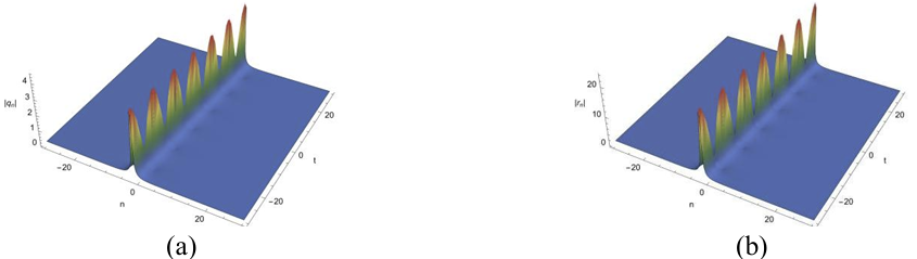
In order to gain a clearer understanding of the obtained solutions and to investigate their dynamical properties, we define
4. Conclusion
In this paper, we focus on the investigation of a two-component integrable semi-discrete coupled local nonlinear Schrödinger equation. Based on the Lax pair, the Darboux transformation (DT) of the system is constructed, and its validity is established through a formal proposition. By choosing appropriate parameters, breather solutions on the zero background are derived. Furthermore, the dynamical behaviors of these solitons are analyzed in detail. The results of this work further reveal novel dynamical distributions of the nonlinear coupled local Schrödinger equation. The proposed approach can also be applied to soliton equations arising from nonlinear local problems in physics and mathematics.
References
[1]. Mark J Ablowitz and Ziad H Musslimani. Integrable nonlocal nonlinear schrödinger equation. Physical review letters, 110(6):064105, 2013.
[2]. Mark J Ablowitz and JF Ladik. Nonlinear differential–difference equa-tions and fourier analysis. Journal of Mathematical Physics, 17(6):1011–1018, 1976.
[3]. Miki Wadati. Transformation theories for nonlinear discrete systems.Progress of Theoretical Physics Supplement, 59:36–63, 1976.
[4]. Mark J Ablowitz and Peter A Clarkson. Solitons, nonlinear evolution equations and inverse scattering, volume 149. Cambridge universitypress, 1991.
[5]. Changbing Hu and Bingtuan Li. Spatial dynamics for lattice differential equations with a shifting habitat. Journal of Differential Equations,259(5):1967–1989, 2015.
[6]. Hao-Tian Wang and Xiao-Yong Wen. Modulational instability, interactions of two-component localized waves and dynamics in a semi-discrete nonlinear integrable system on a reduced two-chain lattice. The Euro-pean Physical Journal Plus, 136(4):461, 2021.
[7]. Roger K Dodd, J Chris Eilbeck, John D Gibbon, and Hedley C Morris.Solitons and nonlinear wave equations. 1982.
[8]. Quanqing Li, Wenbo Wang, Kaimin Teng, and Xian Wu. Ground states for fractional schrödinger equations with electromagnetic fields and crit-ical growth. Acta Mathematica Scientia, 40(1):59–74, 2020.
[9]. Yuen-Ron Shen. Principles of nonlinear optics. 1984.
[10]. Eugene P Bashkin and Alexei V Vagov. Instability and stratification of a two-component bose-einstein condensate in a trapped ultracold gas.Physical Review B, 56(10):6207, 1997.
[11]. William Anderson and Mohammad Farazmand. Shape-morphing reduced-order models for nonlinear schrödinger equations. Nonlinear Dynamics, 108(4):2889–2902, 2022.
[12]. Takayuki Tsuchida, Hideaki Ujino, and Miki Wadati. Integrable semi-discretization of the coupled nonlinear schrödinger equations. Journal of Physics A: Mathematical and General, 32(11):2239, 1999.
[13]. Hai-qiong Zhao and Jinyun Yuan. A semi-discrete integrable multi-component coherently coupled nonlinear schrödinger system. Journal of Physics A: Mathematical and Theoretical, 49(27):275204, 2016.
Cite this article
Guan,L. (2025). Darboux Transformation and Exact Solutions for a Semi-discrete Coupled Local Nonlinear Schrödinger Equation. Theoretical and Natural Science,130,50-56.
Data availability
The datasets used and/or analyzed during the current study will be available from the authors upon reasonable request.
Disclaimer/Publisher's Note
The statements, opinions and data contained in all publications are solely those of the individual author(s) and contributor(s) and not of EWA Publishing and/or the editor(s). EWA Publishing and/or the editor(s) disclaim responsibility for any injury to people or property resulting from any ideas, methods, instructions or products referred to in the content.
About volume
Volume title: The 3rd International Conference on Applied Physics and Mathematical Modeling
© 2024 by the author(s). Licensee EWA Publishing, Oxford, UK. This article is an open access article distributed under the terms and
conditions of the Creative Commons Attribution (CC BY) license. Authors who
publish this series agree to the following terms:
1. Authors retain copyright and grant the series right of first publication with the work simultaneously licensed under a Creative Commons
Attribution License that allows others to share the work with an acknowledgment of the work's authorship and initial publication in this
series.
2. Authors are able to enter into separate, additional contractual arrangements for the non-exclusive distribution of the series's published
version of the work (e.g., post it to an institutional repository or publish it in a book), with an acknowledgment of its initial
publication in this series.
3. Authors are permitted and encouraged to post their work online (e.g., in institutional repositories or on their website) prior to and
during the submission process, as it can lead to productive exchanges, as well as earlier and greater citation of published work (See
Open access policy for details).
References
[1]. Mark J Ablowitz and Ziad H Musslimani. Integrable nonlocal nonlinear schrödinger equation. Physical review letters, 110(6):064105, 2013.
[2]. Mark J Ablowitz and JF Ladik. Nonlinear differential–difference equa-tions and fourier analysis. Journal of Mathematical Physics, 17(6):1011–1018, 1976.
[3]. Miki Wadati. Transformation theories for nonlinear discrete systems.Progress of Theoretical Physics Supplement, 59:36–63, 1976.
[4]. Mark J Ablowitz and Peter A Clarkson. Solitons, nonlinear evolution equations and inverse scattering, volume 149. Cambridge universitypress, 1991.
[5]. Changbing Hu and Bingtuan Li. Spatial dynamics for lattice differential equations with a shifting habitat. Journal of Differential Equations,259(5):1967–1989, 2015.
[6]. Hao-Tian Wang and Xiao-Yong Wen. Modulational instability, interactions of two-component localized waves and dynamics in a semi-discrete nonlinear integrable system on a reduced two-chain lattice. The Euro-pean Physical Journal Plus, 136(4):461, 2021.
[7]. Roger K Dodd, J Chris Eilbeck, John D Gibbon, and Hedley C Morris.Solitons and nonlinear wave equations. 1982.
[8]. Quanqing Li, Wenbo Wang, Kaimin Teng, and Xian Wu. Ground states for fractional schrödinger equations with electromagnetic fields and crit-ical growth. Acta Mathematica Scientia, 40(1):59–74, 2020.
[9]. Yuen-Ron Shen. Principles of nonlinear optics. 1984.
[10]. Eugene P Bashkin and Alexei V Vagov. Instability and stratification of a two-component bose-einstein condensate in a trapped ultracold gas.Physical Review B, 56(10):6207, 1997.
[11]. William Anderson and Mohammad Farazmand. Shape-morphing reduced-order models for nonlinear schrödinger equations. Nonlinear Dynamics, 108(4):2889–2902, 2022.
[12]. Takayuki Tsuchida, Hideaki Ujino, and Miki Wadati. Integrable semi-discretization of the coupled nonlinear schrödinger equations. Journal of Physics A: Mathematical and General, 32(11):2239, 1999.
[13]. Hai-qiong Zhao and Jinyun Yuan. A semi-discrete integrable multi-component coherently coupled nonlinear schrödinger system. Journal of Physics A: Mathematical and Theoretical, 49(27):275204, 2016.