1. Introduction

The logistics function is a typical discrete dynamical system that reflects population growth. Mitchell derived a population growth equation that takes competition for resources into account and gave a model of population growth with a linear effect of resources on population, i.e., logistic growth equation [1-4]. Because environmental changes are periodic on a large time scale, it becomes meaningful to study the periodic stability points of the logistic map. Robert studied the influence of the coefficients of the logistic map on the stability of k-period points and proposed a discriminative method for stable k-period points [4-6]. The Lyapunov exponent is an important method to study the sensitive dependence of the solution on the initial value conditions [4,7-10]. This concept was first introduced in the study of Lorenz attractors and be extended to the general case. Eventually after an algebraic change, it is found that for one-dimensional dynamical systems, Robert's discriminant method and Lyapunov exponent discriminant method are equivalent. However, using the Lyapunov exponent to determine the stability of the periodic points will substantially reduce the computational effort.

2. Method

2.1. Logistics equation

2.1.1. Equation derivation. Phenomena that change in time is often described by differential equations or difference equations. If the current state of the system now depends entirely on the behavior of the previous system, then this system can be described by a class of iterative relations:

where \( x \) _n is the state of the variable at year n, and F maps an interval I into itself. One of the most representative examples is the population growth model. Assuming that at the initial time t₀, the total population is \( x \) ₀, the net population growth rate is \( a \) _net. The relationship between \( x \) _n and \( x \) _n-1 can be portrayed by the equation:

After n iterations, \( {x_{n}} \) = \( a_{net}^{n}{x_{0}} \) , this means that the population will grow exponentially and eventually tends to infinity. This clearly does not correspond to the actual situation. Considering population mortality and the competition due to lack of resources, the actual population growth rate \( a \) _act will gradually tend to zero as the population increases:

N is known as the Environmental Capacity \( ( \) The maximum population that can be achieved under limited environmental resource conditions \( ) \) . Assume that the actual population growth rate \( a \) _act is inversely proportional to the population \( x \) _n, and \( a \) _act must satisfy the condition \( (3)( \) 4 \( ) \) . \( a \) _act can be expressed in the following form:

So that

For the sake of formal simplicity, defining \( x \) _n=N \( y \) _n, \( (6) \) can eventually be reduced to the following form

This is the standard logistics equation \( , f(x)=ax(1-x) \) , \( f \) is logistics map.

2.1.2. Population growth and stabilization cycle solution. To consider whether the population will remain stable or become cyclically stable after a certain period, two concepts need to be introduced: fixed point and periodic point. If \( {x^{*}} \) satisfies the condition, \( {x^{*}}=f({x^{*}}) \) , \( {x^{*}} \) is called \( fixed point \) . If \( {x^{*}} \) satisfies the condition, \( {x^{*}}={f^{(n)}}({x^{*}}) \) , \( {x^{*}} \) is called \( n \) - \( periodic point \) . For k-periodic point, considering the set consisting of \( {x_{i}} \) which satisfis:

\( {x_{i+1}}=f({x_{i}}), i=1,2,3,...,n-1 \)

\( {{f^{(n)}}(x_{i}})={x_{i}}, i=1,2,3,...,n-1 \)

Such set is called an \( n-point limit cycle \) . When the population reaches \( {x^{*}} \) , the population will deviate from \( {x^{*}} \) in a short time due to the inertia of population growth. So figureing out whether \( x \) will return to \( { x^{*}} \) or not is an important question. To solve this problem, the concept of stability of fixed point needs to be introduced. If \( x \) deviate away from \( {x^{*}} \) , it can return to \( {x^{*}} \) in successive generations, the \( {x^{*}} \) is called stable. Fixed point can be viewed as 1-periodic point, so the remaining part will only discuss the case of n-period points. From the point of view of dynamical systems, \( \lbrace {x_{n}}\rbrace _{n=1}^{∞} \) forms a sequence, which \( {x_{n}}={{f^{(n)}}(x_{1}}) \) . For k-period point \( {x_{1}} \) , it generates a sequence with the form \( X=\lbrace {x_{1}}{,x_{2}},{x_{3}},...,{x_{k-1}},{x_{1}}{,x_{2}},{x_{3}},...,{x_{k-1}},...\rbrace \) . To study the stability of \( { x_{1}} \) , adding a certain perturbation \( d \) to \( { x_{1}} \) , letting \( x_{1}^{ \prime }={ x_{1}}+d, \) then \( x_{1}^{ \prime } \) generates a new sequence \( Y=\lbrace x_{1}^{ \prime },x_{2}^{ \prime },x_{3}^{ \prime },...,x_{n}^{ \prime },x_{n+1}^{ \prime },...\rbrace \) , \( x_{n}^{ \prime }={f^{(n)}}(x_{1}^{ \prime }) \) . So, studying the stability of \( { x_{1}} \) is equivalent to studying whether the sequence \( Y \) converges to \( X \) . That is:

\( {{f^{(n)}}(x_{k}})-{f^{(n)}}(x_{k}^{ \prime })→0 as k→∞ \)

From the above, \( X \) is a stable n-point limit cycle if each \( {x_{n}} \) is stable fixed point of \( {f^{(n)}} \) .

For studying the stability of the fixed points of the mapping \( {f^{(n)}} \) , May [4] gives a discriminant method.

\( {x^{*}} is a fixed point of {f^{(n)}}, if |{\frac{d}{dx}f^{(n)}}({x^{*}})| \lt 1, then {x^{*}} is stable. \)

They derived the criterion by the linearization idea. The same conclusion will be obtained by applying Lyapunov exponent.

2.2. Lyapunov exponent

2.2.1. Sensitive dependence on the initial condition. Dynamical systems mostly describe the variation of a variables respect to time. If the solution of the differential equation can be obtained, the state of the variables at time \( t \) can be predicted. Expressing the equation \( x \) _n+1= \( a \) _net \( x \) _n \( (1-x \) _n \( ) \) in the form of differential equation \( \frac{dN}{dt}=aN(1-N) \) , it is easy calculate the analytical solution \( x(t) \) . The curve of \( x(t) \) in the phase plane is called a trajectory and if a point is on this curve, the state of this point at time t can be predicted. But in the real world, there is always an error between the measured value and the exact value due to the accuracy of the measuring instrument. If the solution of the equation is calculated by using the measured values, the measured orbit will deviate from the actual orbit. So, to use the measured track to predict the future state, it is necessary to consider one question - if the initial value deviates from the original value, can the error between the measured trajectory and actual trajectory be kept within a very small range? This phenomenon in which the solution changes dramatically due to a change in the initial measurement conditions is called sensitive dependence on the initial condition. Lyapunov's exponent is possible to discriminate whether the solution is sensitive to the initial value condition.

2.2.2. Lyapunov exponent. This concept was first discovered while studying the Lorenz model.

δ \( (t) \) denotes the distance between two trajectories at time \( t ( \) figure 1 \( ) \) .

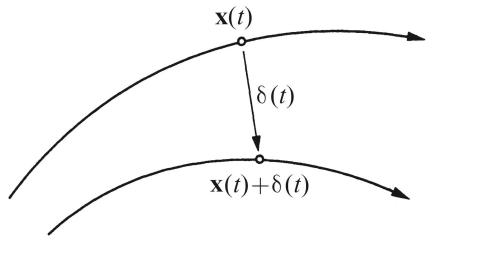
Figure 1. the distance between two trajectories at time \( t \) .

If plot \( ln|δ(t)| \) versus \( t \) , it can be clearly found that a curve which is close to a straight line with a positive slope--λ. According to the graph \( ( \) figure 2 \( ) \) , an equation can be obtained for δ \( (t) \) with respect to \( t \) .

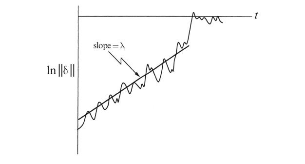
Figure 2. The graph of \( ln|δ(t)| \) about \( t \) .

After algebraic deformation

λ is called the Lyapunov's exponent. Due to the properties of the exponential function, δ \( (t) \) has a fast growth rate whenλis positive and it tends to infinity when t tends to infinity. That means \( {C_{1}} \) does not converge to \( {C_{2}} \) . This makes it impossible to predict the actual state from the measured trajectory.

The Lyapunov's exponent is very useful in the problem of determining the dependence of the trajectory on the initial conditions. Observing Figure 1, the distance between the two trajectories is smaller at one time and bigger at another time. Averaging \( ln|δ(t)| \) over \( t \) can help to measure the average separation of the two trajectories. The linear relationship between \( ln|δ(t)| \) and \( t \) is obtained by averaging \( ln|δ(t)| \) over \( t \) , and can find the finger of λ. Being inspired by this example, the strict definition of Lyapunov exponent and calculation formula of it is given as follow.

Definition: Lyapunov's exponent denotes the numerical characteristics of the average exponential dispersion rate of adjacent trajectories in phase space.

For a one-dimensional discrete dynamical system, the calculation of Lyapunov exponent is derived as follows:

Consider two systems:

\( {x_{n+1}} \) = \( F({x_{n}}) \) and \( {y_{n+1}} \) = \( F({y_{n}}) \)

with small errors in initial conditions \( |{x_{0}}-{y_{0}}| \lt ε \)

After one iteration, \( |{x_{1}}-{y_{1}}|=|F({x_{0}})-F({y_{0}})|=\frac{|F({x_{0}})-F({y_{0}})|}{|{x_{0}}-{y_{0}}|}|{x_{0}}-{y_{0}}| \) since \( |{x_{0}}-{y_{0}}| \lt ε \) ,

\( \frac{|F({x_{0}})-F({y_{0}})|}{|{x_{0}}-{y_{0}}|}|{x_{0}}-{y_{0}}|≈{F^{ \prime }}({x_{0}})|{x_{0}}-{y_{0}}| \)

After n iterations,

\( |{x_{n}}-{y_{n}}|≈|\prod _{i=0}^{n}{F^{ \prime }}({x_{i}})||{x_{0}}-{y_{0}}| \)

To ensure a strong separation, \( δ(n)=|{x_{n}}-{y_{n}}| \) should grow exponentially. So

In the discrete case, the time is taken as positive integer. Imitating equation \( (9) \) , the equation \( (10) \) can be rewritten as \( |lnδ(n)|=\frac{\sum _{i=1}^{n}ln|{F^{ \prime }}({x_{i}})|}{n}n+lnδ(0) \) , furthermore, \( |δ(n)|=|δ(0)|{e^{\frac{\sum _{i=1}^{n}ln|{F^{ \prime }}({x_{i}})|}{n}n}} \) . \( {λ_{n}}=\frac{\sum _{i=1}^{n}ln|{F^{ \prime }}({x_{i}})|}{n} \) measures the average degree of separation after n iterations. To get the behavior of the two trajectories as time tends to infinity, \( \underset{n→∞}{lim}{|δ(n)|}=\underset{n→∞}{lim}{|δ(0)|{e^{{nλ_{n}}}}}=|δ(0)|{e^{nλ}} \) , which \( λ \) = \( \underset{n→∞}{lim}{\frac{\sum _{i=1}^{n}ln|{F^{ \prime }}({x_{i}})|}{n}} \) is the Lyapunov exponent of system. \( λ \) denotes the average degree of exponential separation caused by each iteration of the system over multiple iterations. \( When λ \lt 0 \) , two adjacent points finally coincide after infinite iterations, which implies stability and cyclicality. When \( λ \gt 0 \) , two adjacent points are separated after infinite iterations, which implies local instability.

3. Result----Applying the Lyapunov’s exponent

3.1. K-periodic point

From the previous discussion it is clear that studying the stability of the k-periodic point of the logistics function \( {x_{n+1}} \) = \( F({x_{n}}) \) , which \( F(x)=ax(1-x) \) , is equivalent to studying the stable solution of the equation \( {x_{n+1}} \) = \( {F^{(k)}}({x_{n}}) \) .

From equation 4 ( \( {x^{*}} is a fixed point of {f^{(n)}}, if |{\frac{d}{dx}f^{(n)}}({x^{*}} )| \lt 1, then {x^{*}} is stable). \) If \( {x^{*}} \) is a k-periodic point, F has to satisfy \( |{\frac{d}{dx}F^{(k)}}({x^{*}})| \lt 1 \) . There is another way to determine the stability of point \( {x^{*}} \) by using the Lyapunov exponent, which \( λ \) = \( \underset{n→∞}{lim}{\frac{\sum _{i=1}^{n}ln|{F^{ \prime }}({x_{i}})|}{n}} \) . Because the \( {x^{*}} \) is the k-periodic, \( {F^{ \prime }}({x_{i}}) \) has only a finite number of values \( \lbrace {F^{ \prime }}({x_{i}})\rbrace _{i=0}^{k-1} \) , for \( {x_{i}}={F^{(i)}}({x^{*}}) \) , and \( λ=\frac{\sum _{i=0}^{k-1}ln|{F^{ \prime }}({x_{i}})|}{k} \) .

\( |{{F^{(k)}}^{ \prime }}（{x^{*}} ）| \lt 1⇔|\prod _{i=0}^{k-1}\frac{d}{dx}F({x_{i}})| \lt 1⇔|\sum _{i=0}^{k-1}ln{(\frac{d}{dx}F({x_{i}}))}| \lt 0⇔|\frac{\sum _{i=0}^{k-1}ln|{F^{ \prime }}({x_{i}})|}{k}| \lt 0 \)

\( ⇔λ \lt 0 \)

3.2. Two equivalent determinations

① \( Assume {x^{*}} is a k-period point of F, if |{\frac{d}{dx}F^{(k)}}({x^{*}})| \lt 1 \) , then \( {x^{*}} \) is the stable k-period point of \( F \) .

\( ⇔ ②Assume {x^{*}} is a k-period point of F, if λ \lt 0 \) , then \( {x^{*}} \) is the stable k-period point of \( F \) .

Using the Lyapunov exponent to determine the stability of k-period points can significantly reduce the computational effort. Taking logistics function as an example, \( F(x)=ax(1-x) \) is a quadratic function with a single peak, which becomes a \( 2k \) -th polynomials with \( 2k \) peaks after \( k \) iterations. In computing \( {\frac{d}{dx}F^{(k)}}({x^{*}} ) \) , it is necessary to derive the 2 \( k \) -th polynomial function and perform \( {2k^{2}}+1 \) times multiplication and \( 2k-1 \) times addition, so the total number of operations is equal to \( O({k^{2}}) \) . If the Lyapunov exponent is used to perform the calculation, only the derivative of the quadratic function is needed, then \( \lbrace {x_{i}}\rbrace _{i=0}^{k-1} \) is calculated by \( k-1 \) times multiplication and addition, and finally \( \lbrace {x_{i}}\rbrace _{i=0}^{k-1} \) is brought into the formula \( λ=\frac{\sum _{i=0}^{k-1}ln|{F^{ \prime }}({x_{i}})|}{k} \) for \( k \) times multiplication and \( 2k-1 \) addition. The total number of operations is equal to \( O(k) \) . From Table 1, obviously the calculation of the Lyapunov exponent is much less computationally intensive.

Table 1. Comparison of the computational effort of the two algorithms.

4. Conclusion

An important segment of the logistics map research problem is to study the effect of parameter changes on the behavior of the dynamical system [4]. It is necessary to find the parameter critical values \( ( \) the parameter value that changes the equilibrium point from stable to unstable \( ) \) by determining the stability of many periodic points. Applying the Lyapunov exponent to determine the stability of the periodic point will reduce the computational effort to a great extent.

References

[1]. Feigenbaum, Mitchell J. "Quantitative Universality for a Class of Nonlinear Transformations." Journal of Statistical Physics 19.1 (1978): 25-52. Web.
[2]. May, Robert M. "Simple Mathematical Models with Very Complicated Dynamics." Nature (London) 261.5560 (1976): 459-67. Web.
[3]. May, Robert M. "Biological Populations Obeying Difference Equations: Stable Points, Stable Cycles, and Chaos." Journal of Theoretical Biology 51.2 (1975): 511-24. Web.
[4]. Hirsch, Morris W.; Smale, Stephen, and Devaney, Robert L. Differential Equations, Dynamical Systems, and an Introduction to Chaos (Third Edition). Academic, 2013. Web.
[5]. Li, Tien-Yien, and James A. Yorke. "Period Three Implies Chaos." The American Mathematical Monthly 82.10 (1975): 985-92. Web.
[6]. Zhang, Cheng. "Period Three Begins." Mathematics Magazine 83.4 (2010): 295-97. Web.
[7]. Lorenz, Edward N. "The Problem of Deducing the Climate from the Governing Equations." Tellus 16.1 (1964): 1-11. Web.
[8]. Barreira, Luís. Lyapunov Exponents. Springer International, 2017. Web.
[9]. Barreira, Luis, and Pesin, Ya. B. Lyapunov Exponents and Smooth Ergodic Theory. AMS, 2015. Web.
[10]. Lian, Zeng, and Lu, Kening. Lyapunov Exponents and Invariant Manifolds for Random Dynamical Systems in a Banach Space. American Mathematical Society, 2010. Web.
Cite this article
Yang,Z. (2023). A criterion of periodic point stability based on Lyapunov exponent. Theoretical and Natural Science,10,85-90.
Data availability
The datasets used and/or analyzed during the current study will be available from the authors upon reasonable request.
Disclaimer/Publisher's Note
The statements, opinions and data contained in all publications are solely those of the individual author(s) and contributor(s) and not of EWA Publishing and/or the editor(s). EWA Publishing and/or the editor(s) disclaim responsibility for any injury to people or property resulting from any ideas, methods, instructions or products referred to in the content.
About volume
Volume title: Proceedings of the 2023 International Conference on Mathematical Physics and Computational Simulation
© 2024 by the author(s). Licensee EWA Publishing, Oxford, UK. This article is an open access article distributed under the terms and
conditions of the Creative Commons Attribution (CC BY) license. Authors who
publish this series agree to the following terms:
1. Authors retain copyright and grant the series right of first publication with the work simultaneously licensed under a Creative Commons
Attribution License that allows others to share the work with an acknowledgment of the work's authorship and initial publication in this
series.
2. Authors are able to enter into separate, additional contractual arrangements for the non-exclusive distribution of the series's published
version of the work (e.g., post it to an institutional repository or publish it in a book), with an acknowledgment of its initial
publication in this series.
3. Authors are permitted and encouraged to post their work online (e.g., in institutional repositories or on their website) prior to and
during the submission process, as it can lead to productive exchanges, as well as earlier and greater citation of published work (See
Open access policy for details).