1. Introduction

1.1. The discovery of exoplanets outside solar system

Exoplanet is the most important field in astronomy, as planets are nurseries of lives in the Universe. In 1995, Michael Mayor and Didier Queloz discovered the first exoplanet around a Sun-like star in Pegasus constellation. Their new findings show a wide diversity of planetary systems, enhancing our understanding of planets beyond our Solar system. This is a promising milestone to searching for lives in the Universe, awarded the Nobel Prize in physics in 2019.

Thanks to the development of technology, the detections of exoplanets growth rapidly in the past three decades. Nowadays, over 5,000 exoplanets have been confirmed (NASA Exoplanet Archive, n.d.). The first successful technique for observing exoplanet is radial velocity method, which measures the systematic Doppler shift of absorption lines on the stellar spectrum if the star wobbling induced by orbital movement of its planet. Radial velocity technique dominated the detections of exoplanets in the first 15 years. Another important technique is exoplanetary transits, which measures the periodic decreasing of stellar brightness when planets transit the surface of their host stars in our sight of view. Kepler space telescope, launched in 2009, was a dedicate observatory for the survey of planetary transits with high precision, yielding thousands of detections in its lifetime. Besides the two main technique, other methods, such as gravitational microlensing, direct imaging, timing variations and astrometry, have contributed around 200 detections of exoplanets. So far, transits and radial velocity methods still contribute the most to exoplanets discovery.

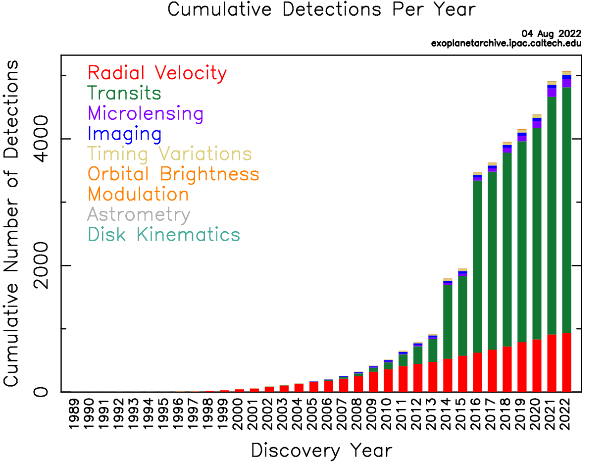
Figure 1. Cumulative discovery of exoplanets using different methods per year. In 21st century, most exoplanets are discovered through transits [1].

1.2. The diversity of exoplanets

The environment and location of a planet are crucial factors for it to be habitable. Exoplanets are classified based on their size, composition, location, and density. The most commonly used categorization for exoplanets is Gas-Giant (large planets composed of helium of hydrogen), Neptunian (planets that similar in size with Neptune or Saturn), super-Earth (planets that heavier than Earth but lighter than gas giant, it can be consisting of rock, ice, or gas), and terrestrial (rocky planets that between half of Earth’s size to twice its radius). The specific type of them can be distinguished based on different features like density and radius. For instance, in Figure 2, the green cluster on the right side can be categorized into Gas-Giant or super-Earth according to their density, and the dispersed population on the left side is considered as Earth Planet, while in Figure 3 the type of a star can be classified according to its mass-radius ratio.

Figure 4 offers a more direct view of exoplanets classification based on mass and radius. The reference planets in the solar system are marked. Several exoplanets system is included as example: TRAPPIST-1 which is famous for its earth-like rocky planets; Kepler-10b that contains a super-Earth; WASP-39b for its watery Saturn… Scholars can analyse those samples to determine the habitability of each exoplanet.

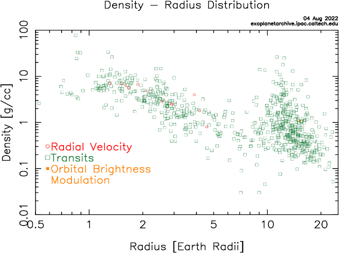
Figure 2. The distribution of exoplanets on radius and density. The size of exoplanets can range from 0.5 \( {R_{Earth}} \) to more than 20 \( {R_{Earth}} \) . The density of those samples is also in a wide range [2].

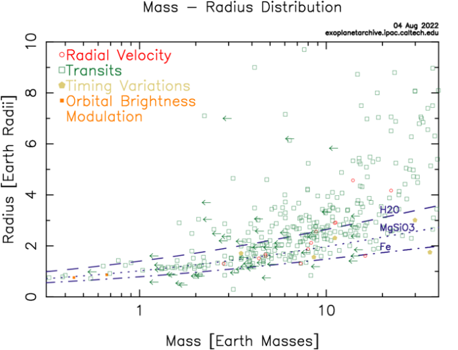
Figure 3. Mass-Radius Distribution of rocky exoplanets. Most of them got mass greater than Earth [3].

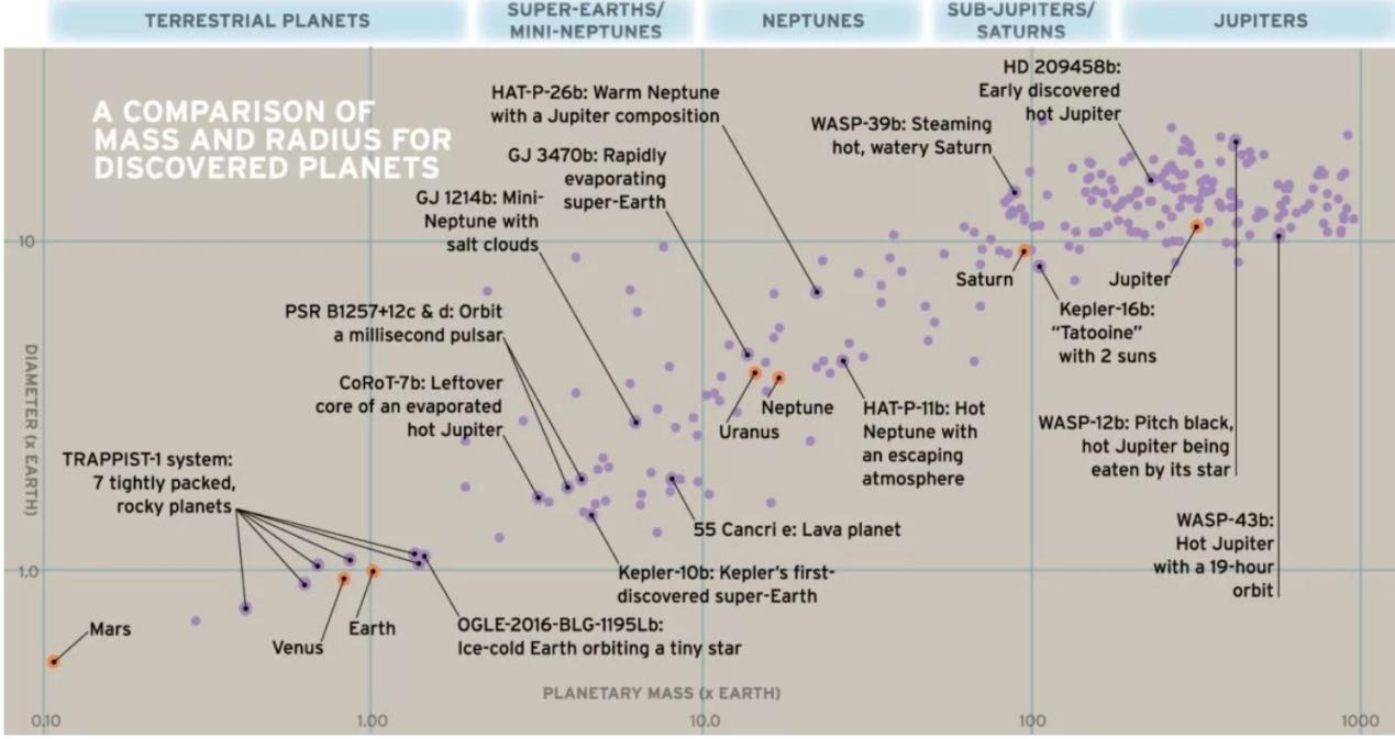
Figure 4. Classification of exoplanets based on their size and mass: Terrestrial planets, super-earths, Neptune’s, Sub-Jupiter/Saturn, and Jupiter [4].

Despite of those ordinary planet types in solar system, some exoplanets have more unique feature that changes people’s understanding of planet’s formation process. In 1995, Mayor and Queloz discovered first exoplanet called 51 Pegasi b around a sun-like star. It is a gas giant that has half of Jupiter’s size but orbital period only 4 days for its close distance to host star. The discovery of 51 Pegasi b changes public’s view in how a planet form. As Figure 5 shown, similar planets found after it are thus categorized as Hot Jupiter---celestial bodies which have period less than 10 days and mass 25% larger than our Jupiter.

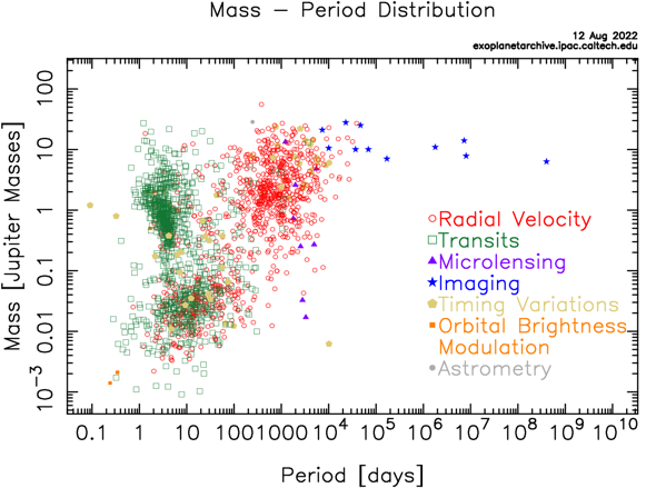
Figure 5. The mass-period distribution of exoplanets founded. The green population on the left side of the graph is hot Jupiter group [5].

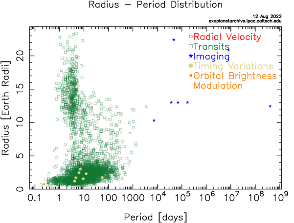
Figure 6. Radius-Period Distribution of exoplanets. Clearly two groups are shown. Most of observations of radius of exoplanets are derived from transits. [6, 7].

1.3. Habitability of exoplanets

Planets need to satisfy several prerequisites to be habitable. First, its configuration should be similar to Earth. Second, the environment of the planet should be suitable for the existence of liquid water. Lastly, it should have proper surface temperature, which means proper distance to its host star. In Figure 7, objects on the left of red zone represents planets which get radiation more than Venus in 1 million years ago (recent Venus), while objects on the right of dark green zone represents planets which get radiation less than Mars in 3.8 billion years ago.

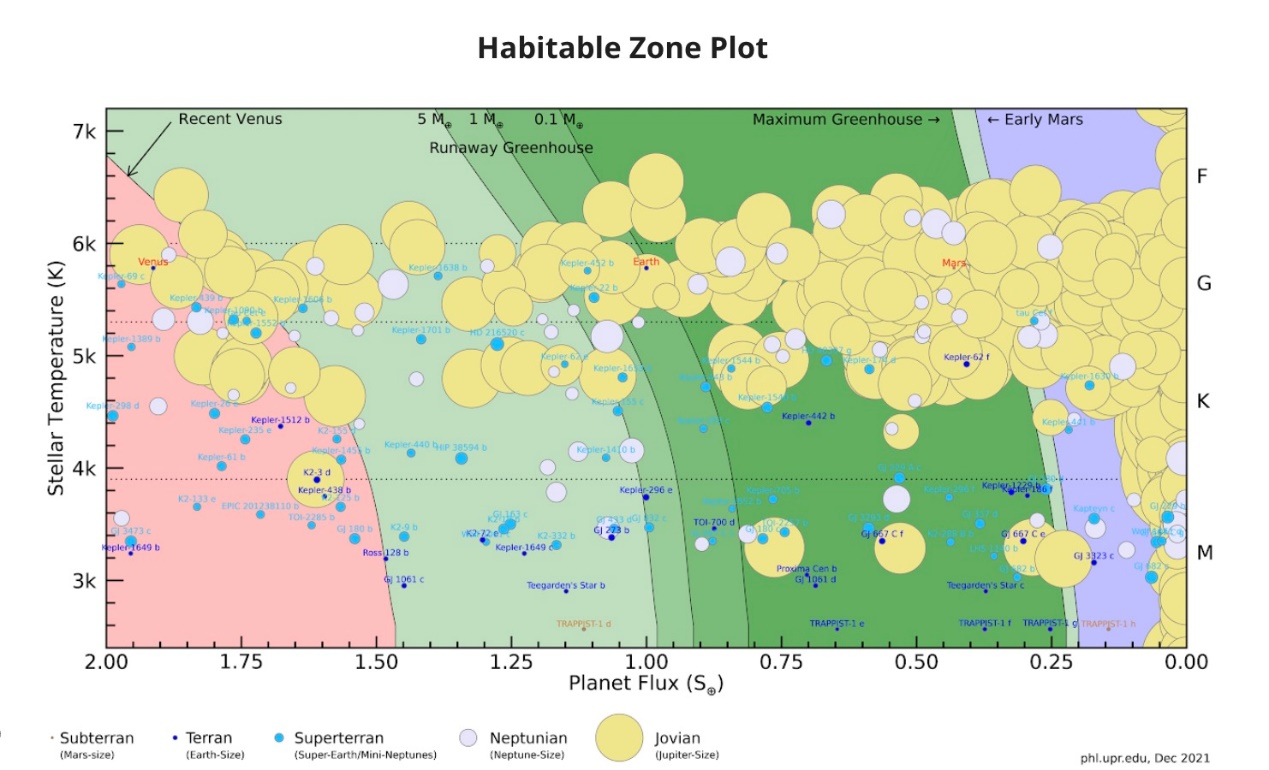
Figure 7. Habitable Zone under solar system reference scale [8].

Planets which concentrated at the green zone have chance to be considered as habitable. However, most of them are Jovian planets that consist of gas, which means they are already excluded from habitable candidates.

For planets inside the green zone, they receive proper amount of radiation from host star. Thus, their average surface temperature is inacceptable range --- not too hot or too cold. Also, the difference between their daily maximum and minimum temperature will not be severe for water to be vaporized or freeze. Thus, planets in this zone can host liquid water.

Another important factor in deciding planets’ surface temperature is the luminosity of the host star and the percent of energy the planet gets.

1.4. An introduction to Alpha Centauri, the closest system to our Solar System

Alpha Centauri is a gravitationally bound system of the closest stars and planets to the Solar System at 4.37 light-years (1.34 parsecs) from the Sun. If there exist habitable planets, they will be our closest neighbours.

It consists of three stars---two sun-like stars (Rigil Kentaurus and Toliman --- which refer to Alpha Centauri A and Alpha Centauri B) and one red dwarf called Proxima. Alpha Centauri A is a yellowish star with mass slightly greater than the sun and 1.5 times brighter, while Alpha Centauri B is less massive and has half brightness of the sun. They are about 5-6 billion years old, a little older than the sun.

As Figure 8 shown, Alpha Centauri AB consists of two close stars and Proxima is far away from it. The semi-major axis of Proxima orbits to Centauri AB is 8700 AU as Table1 shown. However, the semi-major axis of Centauri AB itself is only 23.3 AU, which means the distance between Proxima, and Centauri AB is long.

Figure 8. The location of Alpha Centauri AB and orbit of Proxima.

Table 1. Parameters of Proxima.

So far, a planet around Proxima Centauri had been discovered in 2016 through radial velocity method. This planet raises our interest to investigate the situation of Alpha Centauri system.

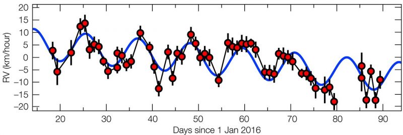
Figure 9. How the motion of Proxima Centauri towards and away from Earth is changing with time over the first half of 2016 [9].

That planet, as called Proxima Centauri b, is classified as Earth-like planet. It’s mass equals 1.27 \( {M_{earth}} \) and size 1.08 \( {R_{earth}} \) . This planet is in the habitable zone of its host star and thus possible for the existence of liquid water.

1.5. Evaluating the possibility of Pandora’s existence in astrophysics perspective

In the movie Avatar, Pandora is described as an Earth-like extra-solar habitable moon in the Alpha Centauri system. It is the fifth moon of the gas giant Polyphemus, which orbits Alpha Centauri A. Since Polyphemus' orbit lies in ACA's habitable zone, appropriately sized planets or moons may have liquid surface water, and therefore support life. The gravity on Pandora is 20% less than Earth, thus results in the birth of strange creatures on it (Wiki Targeted (Entertainment) - The Avatar Wiki, 2022).

In the real world, Pandora cannot exist. In Avatar’s setting, Pandora orbits around a gas giant that has slightly smaller size and higher density than Jupiter in habitable zone of Alpha Centauri A. Based on existing techniques, if there is a planet of such mass in the habitable zone of Alpha Centauri A, scientists can discover it through radial velocity method. However, no planets like Polyphemus are detected so far.

2. Theories

2.1. The law of universal gravitation and the planetary orbit theory

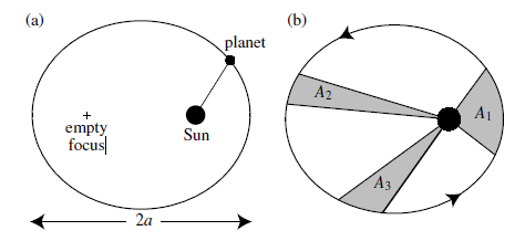
Figure 10. Schematic diagram of Kepler’s laws. Figure (a) is about Kepler’s First Law, and Figure (b) is about Kepler’s Second Law. Kepler’s Third Law cannot be represented by diagrams.

Kepler’s three laws describe how planets orbit the Sun, published by Johannes Kepler between 1609 and 1619. Kepler’s First Law demonstrated that each planet’s orbit about the Sun is an ellipse, and the Sun’s centre is located at one focus of the orbital ellipse. Kepler’s Second Law demonstrates that the imaginary line joining a planet and the Sun sweep equal areas of space during identical time intervals as the planet orbits, which that planets do not move with constant speed along their orbits. Kepler’s Third Law demonstrates that the squares of the orbital periods of the planets are directly proportional to the cubes of the semi-major axis of their orbits, which are presented in an equation,

\( {(\frac{{T_{1}}}{{T_{2}}})^{2}}={(\frac{{a_{1}}}{{a_{2}}})^{3}} \) (1)

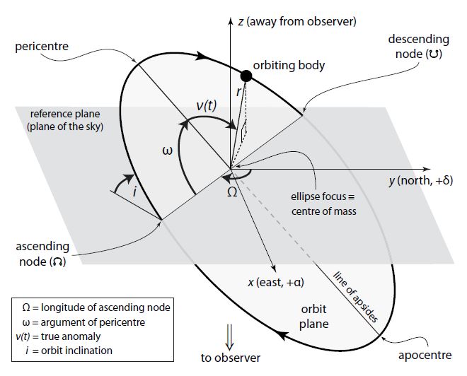
In space, elliptical orbits of planets can be described in the following parameters. The Pericenter and the Apocenter, which is the location of the smallest and the most signific distance between the orbiting body and the central body; the Argument of the Pericenter, \( ω \) , which is the angle from the Ascending Node to the Pericenter; the Eccentricity of the orbit, \( e \) , which is a measure of the orbit’s elongation; the Inclination of the orbit, which is the angle between the orbital plane and a reference plane; the Longitude of the Ascending Node, \( Ω \) , which is the angle from the origin of longitude of the reference plane to the orbit’s Ascending Node; the Longitude of Pericenter, \( ϖ \) , which is the sum of Longitude of Ascending Node and Argument of Pericenter; the Period, \( P \) , which is the time for a planet to complete one orbit; and finally the Semi-major Axis of the orbit, \( a \) , which is 1/2 of the length of the orbit’s major axis.

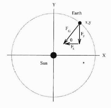
The computer can stimulate the orbit of planets in the Alpha Centauri system by knowing the formula of the velocity and acceleration of the planet in the \( x \) coordinate and \( y \) coordinate direction, also the current position. According to Newton’s law of Gravity and Newton’s Second Law of Motion,

\( {F_{G}}= \frac{G{M_{s}}{M_{p}}}{{r^{2}}} \) (2)

\( \vec{F}=m\frac{{d^{2}}\vec{r}}{{d^{2}}t} \) (3)

The acceleration towards the \( x \) coordinate and \( y \) coordinate of a planet on an orbit at a current position \( (x,y) \) can be expressed as

\( \frac{{d^{2}}x}{{d^{2}}t}=\frac{{F_{G,x}}}{{M_{p}}}=-\frac{G{M_{s}}}{{r^{2}}}cos{θ}=-\frac{G{M_{s}}x}{{r^{3}}} \) (4)

where \( cos{θ}=\frac{x}{r} \) .

\( \frac{{d^{2}}y}{{d^{2}}t}=\frac{{F_{G,y}}}{{M_{p}}}=-\frac{G{M_{s}}y}{{r^{3}}} \) (5)

The velocity toward the \( x \) coordinate and \( y \) coordinate of a planet on an orbit at a current position \( (x,y) \) can be expressed by rewriting the second-order differential equations to first-order differential equations,

\( \frac{d{v_{x}}}{dt}=-\frac{G{M_{s}}x}{{r^{3}}} \) , \( \frac{dx}{dt}={v_{x}} \) (6)

\( \frac{d{v_{y}}}{dt}=-\frac{G{M_{s}}y}{{r^{3}}} \) , \( \frac{dy}{dt}={v_{y}} \) (7)

Before continuing calculation, the units involved should be transferred from SI units, second (s) and meter (m), to larger units, year (yr.), and the distance from Earth to Sun (AU).

On the circle orbit the force caused by centripetal acceleration equals the force caused by the gravitational field, which is

\( \frac{{M_{E}}{v^{2}}}{r}=\frac{G{M_{s}}{M_{E}}}{{r^{2}}} \) (8)

Then,

\( G{M_{s}}={v^{2}}r={r^{2}}{(\frac{2π}{T})^{2}}r=4{π^{2}}(\frac{{AU^{3}}}{{yr^{2}})} \) (9)

Discretize the first-order differential equations to form numeral solutions,

\( \frac{{V_{x, i+1}}-{V_{x, i}}}{Δt}=-\frac{G{M_{s}}{x_{i}}}{{{r_{i}}^{3}}} \) (10)

\( {v_{x, i+1}}={v_{x,i}}-\frac{4{π^{2}}{x_{i}}}{{{r_{i}}^{3}}}Δt \) (11)

\( {x_{i+1}}={x_{i}}+{v_{x, i+1}}Δt \) (12)

\( {v_{y, i+1}}={v_{y,i}}-\frac{4{π^{2}}{y_{i}}}{{{r_{i}}^{3}}}Δt \) (13)

\( {y_{i+1}}={y_{i}}+{v_{y, i+1}}Δt \) (14)

The computer uses the Euler-Cromer method to solve out the values, which is calculating the position and velocity of the planet at step \( i+1 \) according to the position \( (x,y) \) and velocity \( ({v_{x}},{v_{y}}) \) of the planet at step \( i \) . Specifically,

Calculate the distance between the planet and the star,

\( {r_{i}}={({{x_{i}}^{2}}+{{y_{i}}^{2}})^{\frac{1}{2}}} \) (15)

Calculate the velocities on the \( x \) coordinate direction and \( y \) coordinate direction of the planet,

\( {v_{x, i+1}}={v_{x,i}}-\frac{4{π^{2}}{x_{i}}}{{{r_{i}}^{3}}}Δt \) (16)

\( {v_{y, i+1}}={v_{y,i}}-\frac{4{π^{2}}{y_{i}}}{{{r_{i}}^{3}}}Δt \) (17)

Calculate the position of the planet,

\( {x_{i+1}}={x_{i}}+{v_{x, i+1}}Δt \) (18)

\( {y_{i+1}}={y_{i}}+{v_{y, i+1}}Δt \) (19)

As finishing calculating the position and velocities of the planet on step \( i+1 \) , and continue the calculation.

To perform dynamics simulations of multiplanetary systems, we used Mercury, a general software package for N volume fractions. It is used to calculate the orbital evolution of an object moving in the gravitational field of a large centrosome. For example, Mercury can be used to model the motion of planets, asteroids and comets orbiting the sun; Or a system of satellites orbiting planets; Or a system of planets orbiting another star [10]. Furthermore calculation will be discussed in Chapter 3.

2.2. The blackbody radiation theory and the habitability of a planet

A blackbody is an idealized physical body that absorbs all incident electromagnetic radiation, regardless of frequency or angle of incidence. A blackbody emits black-body radiation and can be captured and shown in a black-body spectrum, which it emerges from a system in which matter and radiation are in thermodynamic equilibrium. We approximate that stars shine with the spectrum of a blackbody.

Figure 13. The blackbody spectra, which is the diagram of blackbody radiation, demonstrates the relationships of intensity, frequency and temperature of the radiation.

The curve shown in Figure 4 is known as Planck’s Law,

\( I(λ,T)=\frac{2h{c^{2}}/{λ^{5}}}{{e^{hc/λKT}}-1} \) (20)

and Wein’s Law,

\( {λ_{max}}T=0.29cmK \) (21)

is the relationship between the wavelength at which the peak occurs in wavelength, that the higher the temperature is, the shorter the wavelength occurs, and the higher the frequency of the radiation it achieves. The total energy of the radiation follows Stefan-Boltzmann Law, that the total energy per unit time, per unit surface area, \( E \) , given off by a blackbody is proportional to the fourth power of the temperature, which written in an equation is,

\( E=σ{T^{4}} \) (22)

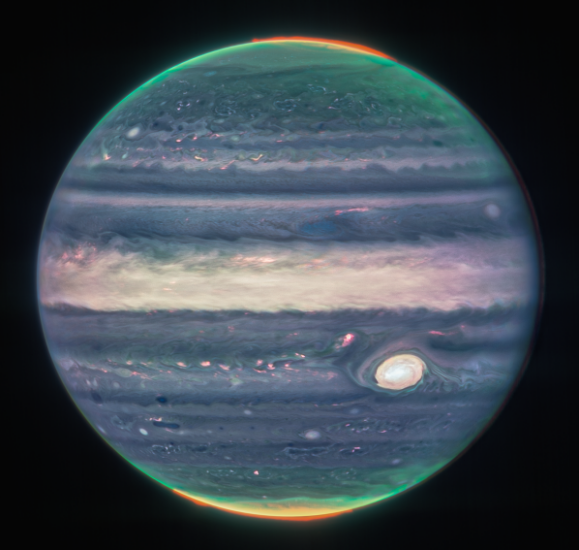
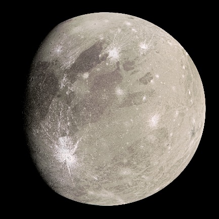
To survive in an environment, the most critical factor is the existence of liquid water. Water is involved in all life activities of carbon-based organisms and the chemical reactions of all organic substances. Therefore, organisms will inevitably be unable to survive if there is no water in an environment. However, the existence of water molecules is not enough to support the production of life. For example, in research by Kivelson et al. [11], the data acquired by the Galileo magnetometer on five passes by Ganymede (see Figure 5), one of the moons of Jupiter, gives evidence to the inductive response model, which demonstrates that there might be an ocean buried beneath Ganymede’s surface. According to another research, the average density of the moon is 1.936 g/cm³, which indicated that Ganymede is composed of nearly equal amounts of rock and water. The latter mainly exists in the form of ice and accounts for 46 – 50 % of the moon’s total mass [12]. Although missions are processed to study Ganymede, it is a fact that there is no life existing on its surface. Therefore, the most fundamental factor in determining planet liability is considering the existence of liquid water.

There are many celestial bodies which contain water molecules in space, such as comets. When those celestial bodies collide into the planet, water will be left on the surface. Planets have long life spans, e.g., Earth has formed 4.5 billion years ag, and research indicates that many planets in the universe have similar or even older age than Earth. Therefore, it is a high probability for planets of being struck by water molecules. Hence, the maintenance of liquid water on the surface of the planet should be taken into consideration.

Planets receive radiation energy from their central stars so they have a specific surface temperature, which might create the right condition for the existence and maintenance of liquid water. However, if the temperature is too high, water will vaporize, and it may escape from the planetary atmosphere. For example, Venus, the second closest planet to the sun in the solar system's eight planets, has an average surface temperature as high as 737K. Venus is similar to Earth in size and mass and is often described as Earth's "sister" or "twin". Research supported that there might be waterbodies which are similar to the oceans on Earth existing in the early ages. However, solar forcing from the rising luminosity of the Sun caused the evaporation of the original water, also causing the decomposition of water vapour into hydrogen and oxygen. Finally, the hydrogen atom escaped to space because of its mass, and the oxygen element was combined with the matter in the crust, resulting in no water molecules existing on the surface of Venus.

If the planet's surface temperature is too low, water will be in a solid state, namely ice, which exists within the planet and cannot support the origin and reproduction of life. Mars, one of the four terrestrial planets in the solar system, has been explored by dozens of unscrewed spacecrafts. According to the natural colour images of Mars captured by Rosetta, it is not difficult to find that there are two polar ice caps which was made largely by water [13]. The radar data of Mars Express and Mars Reconnaissance Orbiter also show large quantities of ice under the surface at both poles and mid-latitude regions [14]. Although it was once widely accepted that Mars has life-supporting qualities, the myth of the Earth-like habitability of Mars was broken in 1925 [15]. Therefore, studying the existence of water is mainly based on the planet's surface temperature.

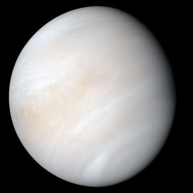
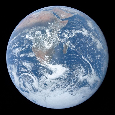
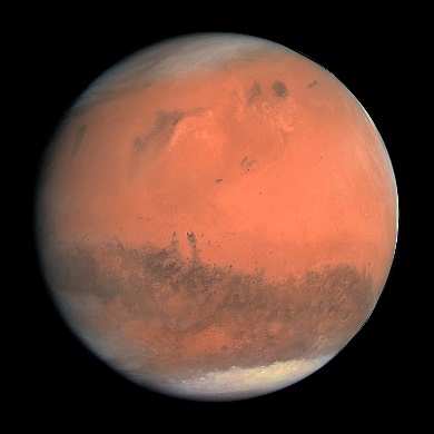
Figure 18. Mars, the fourth planet from the Sun, a terrestrial planet with a thin atmosphere, has a crust composed of elements similar to Earth’s crust. Polar ice caps are found, appeared to be made largely of water, demonstrated that it might be more suited for life in the past. (Mars photographed by Rosetta in 2007)

Three main factors affect the planet's surface temperature – the brightness of the central star, the distance between the planet and the star, and the efficiency of the planet reflecting the star radiation. The habitable zone of stars can be calculated according to these factors, and whether the planet exists in the migration zone can be judged. If the star is approximated as a blackbody, its total radiation luminosity is the product of the star's surface area and the integral intensity of the blackbody radiation frequency, namely:

\( L=(4π{R^{2}}) (σ{T^{4}}) \) (23)

According to the law of inverse square ratio, the energy received by the unit surface area when the planet receives irradiation can be calculated

\( f=\frac{L}{4π{a^{2}}}=\frac{{R^{2}}σ{T^{4}}}{{a^{2}}} \) (24)

Considering that the energy received by the planet is also in the form of blackbody radiation, then

\( {f_{rev}}={f_{emi}} \) (25)

The equilibrium temperature of the planet surface (blackbody temperature) is

\( {T_{eq}}=T\sqrt[]{(\frac{R}{2a})} \) (26)

Because only liquid water can support the generation and reproduction of life, the planet's surface temperature should be between 273 K and 373 K at standard atmospheric pressure, so the range of the star's migration zone can be calculated according to the above formula.

2.3. Milankovitch theory

The Milankovitch cycle describes the collective impact of changes in the Earth's movement on climate over thousands of years. The theory considered that variations in eccentricity, axial tilt and precession is relative to the result in cyclical variations in the intra-annual and latitudinal distribution of solar radiation at the Earth’s surface, causing the change of Earth’s climate patterns.

In research from Petit et al. [16], the data from drilling at Vostok station in East Antarctica (Figure 9), which records the climate changes of Earth in the past 400000 years, shows that the orbital inclination changes over a period of about 40000 years, and the change of orbital eccentricity is about 100000 years, corresponding to the change of global climate, which varies in a period between 100000 years.

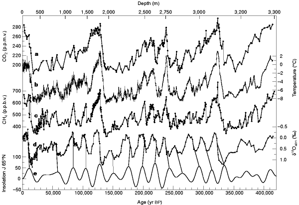
Figure 19. The series measured from the drilling at Vostok with respect to time of: \( C{O_{2}} \) ; Isotopic temperature of the atmosphere; \( C{H_{4}} \) ; \( {δ^{18}}{O_{atm}} \) ; and mid-June insolation at 65 °N. The graph clearly shows the pattern of the changes of climate and Earth’s orbit.

In research from [17], the largest drivers of obliquity variations can extend the outer edge of the habitable zone by preventing runaway glaciation, and the obliquity variations, also orbital variations will have a dramatic impact upon the climate of those planets. In another research by the same researchers and in the same year[18], suggests, that the inclination of the orbit is the main genesis of the instability of the climate, which tend to impair habitability for a planet in a habitable zone. Therefore, the inclination of the orbit of a planet should be taken into consideration when classifying habitable planets.

3. Analysis and simulation

3.1. Habitable zones around stars in α Centauri system

The black body radiation model can be used to describe the radiation of fix stars fairly well. The black body temperature of the star varies with its mass. Planets generates temperature by absorbing the radiation from stars. Thus, planets’ temperatures are closely related to the distance between them and stars. As the image shows below. The green area is the habitable zone. Outside the habitable zone is the blue area, with cooler temperature; and inside is the red area, with higher temperature. Besides, according to Wien’s Law, the higher the blackbody’s temperature is, the shorter its wavelength becomes. This means observing through our eyes, they look blue. While if the star is cooler, it looks redder, corresponding with Figure 21.

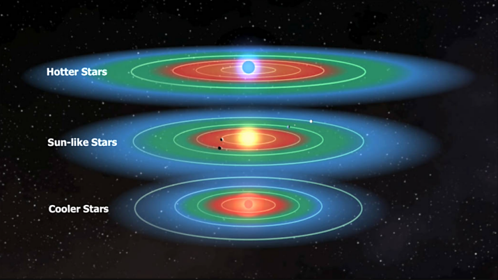
Figure 20. Figure Caption: The figure contrasts the characteristic of stars with different temperatures. As the temperature increases, the colour of the star gets bluer. Correspondingly, its habitable zone locates further from the star.

We’ve already derived the formula

\( a=\frac{R}{2}{(\frac{{T_{s}}}{{T_{p}}})^{2}} \) (27)

Now the affection of blackbody radiation from \( α \) Centauri \( a \) , \( b \) , and \( c \) to the planets can be calculated. Also, the location of habitable zones can be calculated.

Known that the radius of the earth is \( {R_{s}}= \) 6.96×10⁸ m, the radius of \( α \) centauri \( a \) is \( {R_{a}}=1.23 {R_{s}} \) , the radius of \( α \) Centauri \( b \) is \( {R_{b}}=0.84 {R_{s}} \) , the radius of \( α \) Centauri \( c \) is \( {R_{c}}=0.131{ R_{s}} \) . Define that habitable zone are the area that has a temperature between 273 k and 373 k.

Plug the data into the formula, and derive that the habitable zone of \( α \) Centauri \( a \) is between 1.83585×10¹¹ m to 9.8318×10¹⁰ m, the habitable zone of \( α \) Centauri \( b \) is between 1.0265×10¹¹ m to 5.49877×10¹⁰ m, the habitable zone of \( α \) Centauri \( c \) is between 4.87333×10⁹ m to 2.61056×10⁹ m.

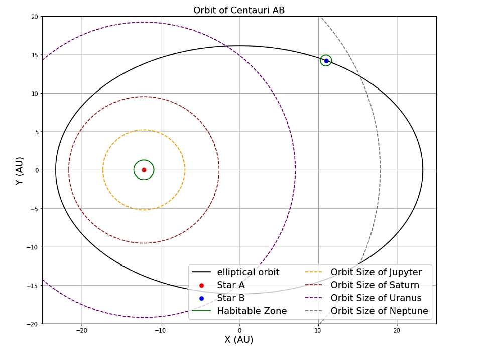
Figure 21. The figure shows the orbit of each planet in the system and their distance from each other.

The result has clearly shown that the habitable zones of \( α \) Centauri \( a \) and \( b \) are relatively small than the orbit size of Jupiter-like planets. So, it denied the possibility that there are planets of Jupiter-mass in the habitable zone. The whole \( α \) Centauri system is like a solar system with two suns, that is to say, two stars in it. When there is only one star, the stability would be what it’s like in the solar system. While now there are two stars, the stability of the planet has to be considered. Mention that here we ignored the Proxima Centauri since its mass is relatively small to \( α \) Centauri \( a \) and \( b \) . It’s more likely to be considered as an isolated star, about 8700 au distance from the \( α \) Centauri system

3.2. Astronomical observations against scenario in film

When a planet orbits a star, despite its relatively small mass, it can have an effect on the star. This effect causes the star to move correspondingly around the centre of mass. In the process of motion, because the celestial body is constantly releasing or reflecting light waves, the Doppler shift occurs. The frequency of light wave of celestial bodies far away from the observation point becomes slow and red shift occurs. And approaching objects become faster and blue shifted. The radial velocity of a star can be quantitatively and accurately analysed by analysing the detected spectrum, thus studying the motion state of a star.

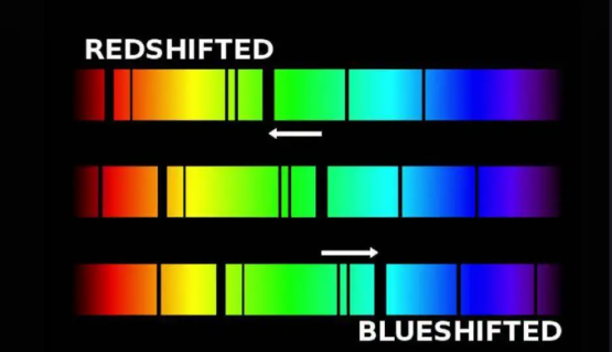
Figure 22. A schematic diagram of blue shift and red shift of stellar spectrum. A blue shift does not mean that the object ends up blue. It just means that the entire spectrum is shifted up in frequency.

(Have Astronomers Ever Observed a Violet Shift Like They Have Blue Shifts and Red Shifts 2013)

Detecting limit:

\( K=28.4{{m_{s}}^{-1}}{(\frac{P}{1yr})^{-\frac{1}{3}}}(\frac{{M_{p}}sin{i}}{{M_{J}}}){(\frac{{M_{⋆}}}{{M_{⊙}}})^{-\frac{2}{3}}} \) (28)

First transmit the time unit to day, the planet’s mass’ unit to earth’s mass, to help with the calculation

\( K=28.4{{m_{s}}^{-1}}{(\frac{P}{365.25day})^{-\frac{1}{3}}}(\frac{{M_{p}}sin{i}}{{317.965M_{e}}}){(\frac{{M_{⋆}}}{{M_{⊙}}})^{-\frac{2}{3}}} \) (29)

Simplify the formula

\( K=0.64{{m_{s}}^{-1}}{(\frac{P}{1day})^{-\frac{1}{3}}}(\frac{{M_{p}}sin{i}}{{M_{e}}}){(\frac{{M_{⋆}}}{{M_{⊙}}})^{-\frac{2}{3}}} \) (30)

Transform the formula and finally derive

\( {M_{p}}sin{i}=\frac{K}{0.64}{{(P)^{\frac{1}{3}}}({M_{⋆}})^{\frac{2}{3}}} \) (31)

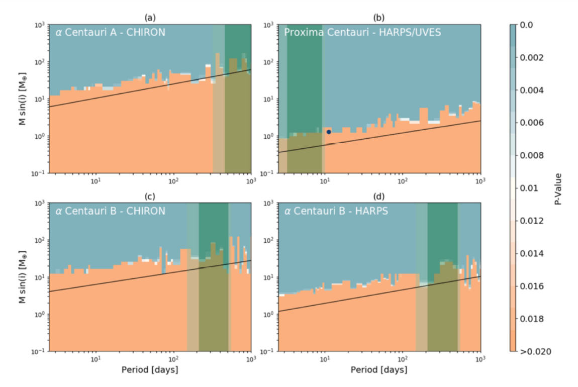
Figure 23. The orange columns represent the mass and period of different planets. The green parts are habitable zones. And the black line represents the detecting limit.

(ShieldSquare Captcha, n.d.)

A research group from Yale University had studied the detecting threshold for the α Centauri system for decades . They estimated the chemical composition of each planet through their similarities to planets in the solar system and then observed their radio velocity. They concluded that there is an Earth-like planet orbiting Proxima Centauri, while they couldn’t find a planet orbiting \( α \) Centauri \( a \) and \( b \) , so they had to derive the detecting limit. According to their study, for \( α \) Centauri \( a \) , the detecting threshold is set as \( K \) >2.5 m/s; for \( α \) Centauri \( b \) , the detecting threshold is set as \( K \) >1 m/s; for Proxima Centauri, the detecting threshold is set as \( K \) >1 m/s.

Thus, we can plug the data into the formula, and obtain that the detecting limit for a Centauri A is about 17.9 Earth mass, the detecting limit for a Centauri B is about 6.3 Earth mass, the detecting limit for Proxima Centauri is about 1.5 Earth mass.

3.3. Temperate planetary orbits around α Centauri A and B

In order to allow lives to appear on a planet, it not only has to be habitable, also the habitable zone has to be stable enough to allow a long-life period to take place. So, stability is also a key element restricting planets’ habitability.

We use a program to simulate the periodic motion of the α Centauri system. In the simulation, we assume that there is one planet that can perfectly fit in α Centauri a’s habitable zone. According to previous calculation about its mass and semimajor axis, the simulation can be quite precise. We set the timestep as 0. 1 days to be as precise as possible. And set the output interval as 100 days, to derive a smooth and continual curve. The whole simulation would calculate the eccentricity, semimajor axis and inclination for each planet in the system. So, we can know the state of the planet exactly at any time. The whole simulation calculates the transition in 10,000,000 days, and that’s about 27397 years, so we can see the periodic variation obviously.

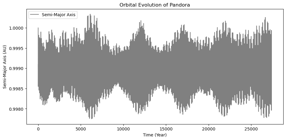
Figure 24. The variation of the semi-major axis.

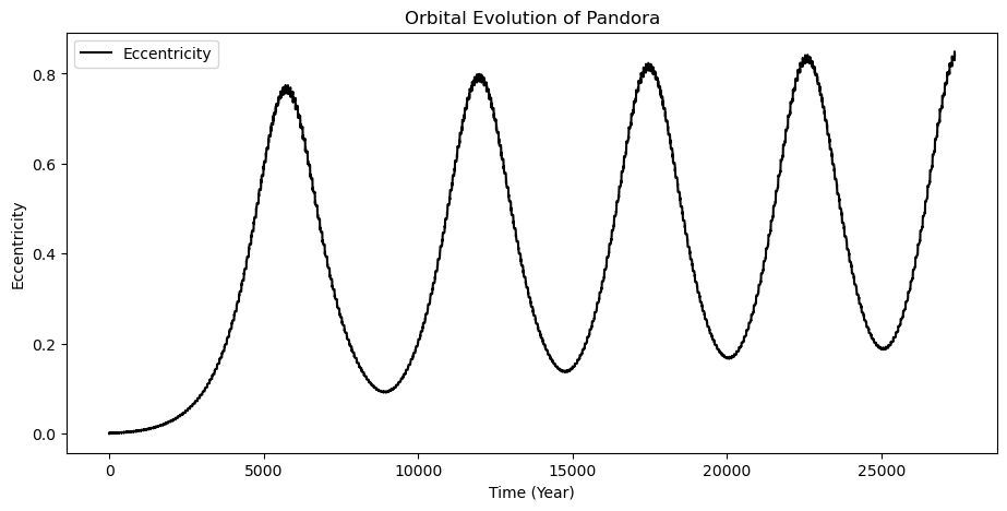
Figure 25. The variation of the eccentricity.

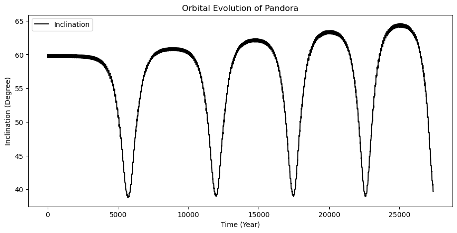
Figure 26. The variation of the inclination.

From the result, we can see that the planet’s semi-major axis has a fluctuation period of about 5000 years. The periods are not exactly the same, but they are quite similar to each other. Each period has many peaks, and the fluctuation is relatively rapid. The range of fluctuation is only about 0.02.

The eccentricity has a period of about 5000 years. The period length decreases a little bit over time. The overall trend increases a little. The periodic variation is obvious. It fluctuates in a range of about 0.8.

The inclination has a period of about 6000 years. The period length also decreases a little over time. The periodic variation is also obvious. The range of fluctuation increases a little bit within a range of about 15 degrees.

Above all, when the inclination rises, correspondingly the eccentricity declines. The inclination and the eccentricity are complementary. That’s consistent with the angular momentum conservation law. And when the inclination is between 65 to 40 degree, the system is relatively stable, and the planet is habitable. With this stable system and periodic feature, we can infer that the planet is habitable.

The movie Avatar described Pandora as a habitable moon of a Jupiter-mass planet While from our research, we can approve that there can be life on the planet. However, it must not be a Jupiter mass planet. One reason is that for one or more than one earth mass planet, the orbit can keep stable. While for a Jupiter mass planet, the stability would be severely influenced, and that may contradict with its high habitability showed in the movie. Another evidence is that the detecting limit for a Centauri A is about 17.9 earth mass, the detecting limit for a Centauri B is about 6.3 earth mass. If there is a Jupiter mass planet existing in the system, it must have already been found. Obviously, there isn’t any relating news till now.

4. Conclusion

This research focuses on the possibility of the virtual planet Pandora being existed and habitable. Researchers introduce the latest results and understanding of exoplanets study and list general types of exoplanets and methods astronomers used to find them. Based on current data, it is impossible for Pandora’s host planet, which should be a gas giant, to exist without being detected. Then researchers then introduce different metrics used to analyse the habitability of planets. By employing calculations according to black body radiation, the requirements for liquid water to maintain on a planet’s surface are shown. Also, according to Milankovitch Theory, the inclination of a planet’s orbit should also be considered when discussing its habitability. Then the researchers did a simulation in Alpha Centauri System and assume an existence of an earth-like planet just like Pandora inside it. The variation in eccentricity and semi-major axis, as well as orbital evolution of Pandora has been analysed. At last, we found that this assumed moon can be habitable, but its host planet should not exist.

References

[1]. NASA Exoplanet Archive. (n.d.). Retrieved September 7, 2022, from https://exoplanetarchive.ipac.caltech.edu/
[2]. NASA Exoplanet Science Institute. (2022, April). Cumulative detection of exoplanets per year. NASA Exoplanet Archive. https://exoplanetarchive.ipac.caltech.edu/exoplanetplots/ exo_dischist_cumulative.png
[3]. NASA Exoplanet Science Institute. (2022, April). Density-Radius Distribution. NASA Exoplanet Archive. https://exoplanetarchive.ipac.caltech.edu/exoplanetplots/exo_densrad.png
[4]. Wiki Targeted (Entertainment). (n.d.). Avatar Wiki. Retrieved September 7, 2022, from https://james-camerons-avatar.fandom.com/wiki/Pandora
[5]. NASA Exoplanet Science Institute. (2022, April). Mass-Radius Distribution of rocky exoplanets. NASA Exoplanet Archive. https://exoplanetarchive.ipac.caltech.edu/exoplanetplots/ exo_massradius.png
[6]. NASA Exoplanet Science Institute. (2022a, April). Mass-Period Distribution of Exoplanets Founded. NASA Exoplanet Archive. https://exoplanetarchive.ipac.caltech.edu/exoplanetplots/ exo_massperiod.png
[7]. NASA Exoplanet Science Institute. (2022c, April). Radius-Period Distribution of Exoplanets. NASA Exoplanet Archive. https://exoplanetarchive.ipac.caltech.edu/exoplanetplots/ exo_radperiod.png
[8]. PHL @ UPR Arecibo - The Habitable Exoplanets Catalog. (n.d.). Retrieved September 7, 2022, from https://phl.upr.edu/projects/habitable-exoplanets-catalog
[9]. Escudé, A. (2016b). The motion of Proxima Centauri Towards and Away from Earth. Europe Southern Observatory.
[10]. Chambers, J. E. (1999). A hybrid symplectic integrator that permits close encounters between massive bodies. Monthly Notices of the Royal Astronomical Society, 304(4), 793–799. https://doi.org/10.1046/j.1365-8711.1999.02379.x
[11]. Kivelson, M., Khurana, K., & Volwerk, M. (2002). The Permanent and Inductive Magnetic Moments of Ganymede. Icarus, 157(2), 507–522. https://doi.org/10.1006/icar.2002.6834
[12]. Springer. Showman, A. P., & Malhotra, A. R. (1999). The Galilean Satellites. Science, 286(5437), 1–84. https://doi.org/10.1126/science.286.5437.77
[13]. Byrne, S., & Ingersoll, A. P. (2003). A Sublimation Model for Martian South Polar Ice Features. Science, 299(5609), 1051–1053. https://doi.org/10.1126/science.1080148
[14]. Holt, J. W., Safaeinili, A., Plaut, J. J., Head, J. W., Phillips, R. J., Seu, R., Kempf, S. D., Choudhary, P., Young, D. A., Putzig, N. E., Biccari, D., & Gim, Y. (2008). Radar Sounding Evidence for Buried Glaciers in the Southern Mid-Latitudes of Mars. Science, 322(5905), 1235–1238. https://doi.org/10.1126/science.1164246.
[15]. Wright, W. H. (1949). Biographical Memoir of William Wallace Campbell, 1862–1938. National Academy of Sciences.
[16]. Petit, J. R., Jouzel, J., Raynaud, D., Barkov, N. I., Barnola, J. M., Basile, I., Bender, M., Chappellaz, J., Davis, M., Delaygue, G., Delmotte, M., Kotlyakov, V. M., Legrand, M., Lipenkov, V. Y., Lorius, C., PÉpin, L., Ritz, C., Saltzman, E., & Stievenard, M. (1999). Climate and atmospheric history of the past 420,000 years from the Vostok ice core, Antarctica. Nature, 399(6735), 429–436. https://doi.org/10.1038/20859
[17]. Deitrick, R., Barnes, R., Quinn, T. R., Armstrong, J., Charnay, B., & Wilhelm, C. (2018). Exo-Milankovitch cycles. I. Orbits and rotation states. The Astronomical Journal, 155(2), 60.
[18]. Deitrick, R., Barnes, R., Bitz, C., Fleming, D., Charnay, B., Meadows, V., ... & Quinn, T. R. (2018). Exo-Milankovitch cycles. II. Climates of G-dwarf planets in dynamically hot systems. The astronomical journal, 155(6), 266.
Cite this article
Ying,H.;Tie,X.;Chen,W.;Wu,W. (2023). Astrophysical investigation on the virtual planet pandora in Avatar film. Theoretical and Natural Science,11,180-198.
Data availability
The datasets used and/or analyzed during the current study will be available from the authors upon reasonable request.
Disclaimer/Publisher's Note
The statements, opinions and data contained in all publications are solely those of the individual author(s) and contributor(s) and not of EWA Publishing and/or the editor(s). EWA Publishing and/or the editor(s) disclaim responsibility for any injury to people or property resulting from any ideas, methods, instructions or products referred to in the content.
About volume
Volume title: Proceedings of the 2023 International Conference on Mathematical Physics and Computational Simulation
© 2024 by the author(s). Licensee EWA Publishing, Oxford, UK. This article is an open access article distributed under the terms and
conditions of the Creative Commons Attribution (CC BY) license. Authors who
publish this series agree to the following terms:
1. Authors retain copyright and grant the series right of first publication with the work simultaneously licensed under a Creative Commons
Attribution License that allows others to share the work with an acknowledgment of the work's authorship and initial publication in this
series.
2. Authors are able to enter into separate, additional contractual arrangements for the non-exclusive distribution of the series's published
version of the work (e.g., post it to an institutional repository or publish it in a book), with an acknowledgment of its initial
publication in this series.
3. Authors are permitted and encouraged to post their work online (e.g., in institutional repositories or on their website) prior to and
during the submission process, as it can lead to productive exchanges, as well as earlier and greater citation of published work (See
Open access policy for details).