1. Introduction

The Stirling approximation is a mathematical tool with applications in probability, statistics, and thermodynamics. In thermodynamics, the Stirling approximation is particularly useful for understanding the concepts of entropy, the flow of entropy, mechanical equilibrium, and processes such as the Joule expansion. These concepts are fundamental to thermodynamics, which seeks to understand the behavior of energy in physical systems.

Entropy is a measure of the disorder or randomness of a system, and it is closely related to the second law of thermodynamics, which states that the entropy of an isolated system will tend to increase over time. The Stirling approximation can be used to estimate the number of possible states of a system, which is related to entropy. Additionally, the flow of entropy is the transfer of entropy between different systems, and it is a key component of thermodynamic processes. Mechanical and thermal equilibrium refers to the state in which the energy or entropy in a system is balanced, and it is also related to the second law of thermodynamics.

One example of a thermodynamic process is the Joule expansion, which involves the expansion of a gas without any temperature change. The Joule expansion is important because it illustrates the relationship between entropy and energy, and it can be used to understand the behavior of complex systems. The Stirling approximation can be applied to the Joule expansion to estimate the change in entropy that occurs during the expansion.

This essay will explore the Stirling approximation and its applications in thermodynamics, including its relationship to entropy, the flow of entropy, and mechanical and thermal equilibrium. It will also discuss the Joule expansion and how it relates to these concepts. It will begin by discussing the history and development of the Stirling approximation and its relationship to the concept of entropy and the number of microstates. Then the essay will introduce the concept of the flow of entropy and its relationship to the Stirling approximation. Next, it will explore the concept of mechanical and thermal equilibrium and its relationship to entropy and the second law of thermodynamics. Finally, there will have some discussion of the Joule expansion and how it illustrates the relationship between entropy and energy.

Overall, this essay seeks to provide a comprehensive understanding of the Stirling approximation, its applications in thermodynamics, and its significance in various fields of study. By exploring the Stirling approximation and related concepts, as well as the Joule expansion, which hope to contribute to a deeper understanding of the fundamental laws of nature and provide valuable insights into the behavior of complex systems and processes.

2. Analysis of Stirling approximation and entropy

2.1. Stirling approximation

Stirling approximation is an approximation for factorials, which to put it mathematically, can be expressed by the following formula.

\( log{(N!)}=NlogN-N \) (1)

This formula can be further transformed into another version

\( log{(N!)}=NlogN(\frac{N}{e}) \) (2)

\( N!={(\frac{N}{e})^{N}}={N^{N}}{e^{-N}} \) (3)

Its derivation can be achieved by approximating the sum over the terms of the factorial with an integral[1], where log(N!) is the sum of log(1)+log(2)+. . . +log(N). The definition of integration is to add all the values together, or the sum of the area under the curve of a function as shown in figure 1.

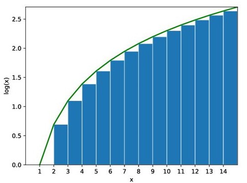
Figure 1. The integration shown in graph [2].

To put it in the formula form

\( \sum _{k=1}^{n}log⁡(k)=\int _{1}^{N}log{(x)}dx=NlogN-N \) (4)

Figure 2 shows that the curve of the computed function by using the Stirling approximation which is marked as a dashed line for nlog(n)-n, matches closely with the function of log(n!) which are the points. As for the solid line, the \( \sqrt[]{2πn} \) is the correction that is put into the formula.

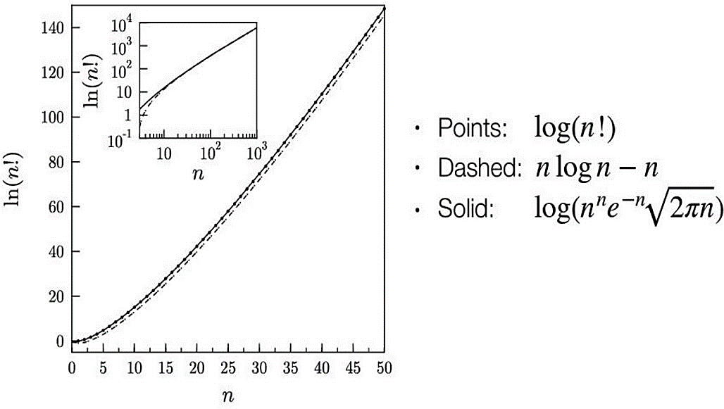
Figure 2. Graph of Stirling approximation [2].

The Stirling approximation is named after the Scottish mathematician James

Stirling, though a related but less precise result was first derived by Abraham de Moivre.[3] The formula he discovered was \( n![constant]{n^{n-\frac{1}{2}}}{e^{-n}} \) . Based on this formula, Stirling was able to show the constant is precisely \( \sqrt[]{2π} \) .

One application of using the Stirling approximation is to count the possibility of placing a certain number of balls randomly into a certain number of baskets.

From figure 3 below, it describes the possible situation of placing 3 balls into

4 baskets. There are 12 possible ways when putting two balls in one basket and one in the other, 4 ways when putting all three balls in one basket, and 4 ways of one ball in one basket only.

Figure 3. The possibility of placing balls.

It is easy to count when the number of balls and baskets is small numbers. When it comes to bigger numbers, the number of possible ways can be calculated by formula. The formula of counting the number of ways can be expressed by (5). In which N represents the number of balls and q is the number of baskets. The Ω(q) here is the number of possible ways of putting balls into the basket, or it can also be referred to as the number of possible states.

To perform the calculation easier using this formula, the Stirling approximation is used to transform this formula into a more convenient form.

\( Ω(q)=\frac{(N+q-1)!}{q!(N-1)!}={(\frac{N+q}{e})^{N+q}}\frac{1}{{(\frac{q}{e})^{q}}}\frac{1}{{(\frac{N}{e})^{N}}}=\frac{({1+ \bar{n} ) ^{(N+q)}}}{{(\bar{n} )^{q}}} \) (5)

\( \bar{n} =\frac{q}{N} \) (6)

In this equation, the calculation is made of only multiplication and exponential, which is an easier calculation than the factorial calculation from the original formula.

After the number of possibilities is calculated, it is easy to derive the value of entropy, as entropy is defined by the formula 7.

\( S={K_{b}}ln⁡(Ω) \) (7)

2.2. Entropy

The definition of entropy is most commonly associated with a state of disorder, randomness, or uncertainty[4]. It can be used to describe how chaotic a system is. As the entropy of a system increases, the system would tend to be more mixed together or evenly distributed.

As the entropy of a system can be calculated this way, it is possible to derive the change in entropy of two connected systems, or the flow of entropy. Figure 4 shown below represents two isolated systems each containing a certain amount of gas, which respectively have the energy E1, E2, and number of states Ω1 and Ω2 individually. When there is a channel created between two systems, as they are connected, gas from either side would flow to the other, according to the second law of thermodynamics and the thermal exchange.

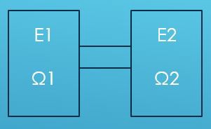
Figure 4. The model of two connected systems.

2.3. Flow of entropy

Equation 8 shows the change of entropy of the entire system when two systems are connected due to the entropy flow. As two systems are connected, the change of energy of one system is the same as the other but with opposite signs, which is equation 9. By combining 8 and 9, it gives 10 which the change of entropy has to be greater or equal to zero since the entropy of an isolated system can never decrease.

When \( (\frac{∂S1}{∂E1}-\frac{∂S2}{∂E2}) \gt 0 \) , the energy would flow from right to left, \( \frac{dS1}{dE1} \gt 0 \) . Vice versa.

Entropy reaches a maximum when \( \frac{dS}{dt}=0 \) or when \( \frac{∂S1}{∂E1}=\frac{∂S2}{∂E2} \) , which indicates that the two systems are equally mixed together and particles are evenly distributed.

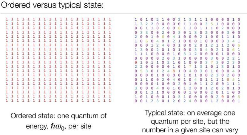
Figure 5(a) shows the ordered state where everything is the same. Yet the typical state on figure 5(b) shows that all different numbers are evenly mixed in the system, and as the number of state Ω increases, the numbers are distributed more uniformly and eventually reach equilibrium.

\( \frac{d{S_{total}}}{dt}=\frac{∂S1}{∂E1}\frac{dE1}{dt}+\frac{∂S2}{∂E2}\frac{dE2}{dt} \) (8)

\( \frac{dE2}{dt}=-\frac{dE1}{dt} \) (9)

\( \frac{d{S_{total}}}{dt}=(\frac{∂S1}{∂E1}-\frac{∂S2}{∂E2})\frac{dE1}{dt}≥0 \) (10)

Therefore, the temperature can be defined as equation 11. The entropy is maximized when \( \frac{∂S1}{∂E1}=\frac{1}{T1}=\frac{1}{T2}=\frac{∂S2}{∂E2} \) . In this case, dE1 can be identified as the heat \( \bar{d}Q \) added to system 1. Equation 11 summarizes that the change in entropy can be described as the heat added and rethermalized over the temperature, in which the ∆s can be determined from the measurements of energy flow of temperature changes.

By recalling the Ω(E) that was able to be calculated using the Stirling approximation, here it represents the number of ways to share the available energy.

\( dS1=\frac{\bar{d}Q1}{T1} \) (11)

2.4. Mechanical and thermal equilibrium

Thermal equilibrium is achieved when two systems in thermal contact with each other cease to exchange energy by heat. If two systems are in thermal equilibrium their temperatures are the same. The word equilibrium implies a state of balance. In an equilibrium state, there are no unbalanced potentials (or driving forces) within the system. A system that is in equilibrium experiences no changes when it is isolated from its surroundings[6].

The first law of thermodynamics states the total energy of the system is conserved, as equation 12 states that the change of total energy is the sum of the heat energy and the work done by the system, in which the heat energy is the change of entropy times temperature, and the work done is a change of volume times pressure which the result gives out equation 15. Therefore, the change of entropy can be expressed as equation 16.

\( du=\bar{d}Q+\bar{d}w \) (12)

\( \bar{d}Q = TdS \) (13)

\( \bar{d}w = -PdV \) (14)

du \( = \) TdS – PdV (15)

\( dS=\frac{1}{T}du+\frac{P}{T}dV \) (16)

Equation 10 above can also replace the E with V, which is equation 17, from what was just derived earlier, equation 17 can get equation 18, which in this form, it shows that the equilibrium is reached when \( \frac{P1}{T1}=\frac{P2}{T2} \) and \( \frac{1}{T1}=\frac{1}{T2} \) for S_total=0.

\( \frac{d{S_{total}}}{dt}=(\frac{∂S1}{∂V1}-\frac{∂S2}{∂V2})\frac{dV1}{dt} \gt 0 \) (17)

\( \frac{d{S_{total}}}{dt}=(\frac{P1}{T1}-\frac{P2}{T2})\frac{dV1}{dt} \gt 0 \) (18)

From the second law of thermodynamics, the total amount of entropy is always increasing, and for the systems from the previous part, the total change of entropy is the sum of the change of entropy in each system, which combines with equations 16,17 and 18 previously derived, the total change of entropy in this model can be expressed as equation 19, and as the system reaches equilibrium when it equals 0, the system would have thermal equilibrium when T1 = T2, and mechanical equilibrium when P1 = P2.

\( \frac{d{S_{total}}}{dt}=(\frac{1}{T1}-\frac{1}{T2})dE1+(\frac{P1}{T1}-\frac{P2}{T2})dV1≥0 \) (19)

2.5. Joule expansion

A Joule expansion is an example of an irreversible process. In a Joule expansion, a gas expands irreversibly from a volume V1 into a volume V2 (initially a vacuum), so that the total volume of the gas after expansion is V1 +V2. The system is thermally isolated and no external work is done on the gas[7].

By using the model of a two-container system, only one container would be filled with gas initially and with a piston between them, and as the gas in the system expands, the piston moves towards the other side and the volume increases. However, during the process, no energy is transferred, and the temperature is the same at the beginning and the end.

For an irreversible process, the entropy always increases, in which ∆S > 0, which ∆s here is only a function of the initial equilibrium state and the final equilibrium state. For a mono-atomic gas, the energy is shown as equation 20, and it can transform to 21, and from 22 which is the ideal gas law, it can be derived to 23. By combining with equation 16, they get equation 24. Then the entropy can also be calculated by integrating the equation of dS, which the result would be equation 25, where C is a constant after integration. From the earlier expression of entropy in equation 7, the number of possible states can be alternatively expressed as equation 26, by combing it with 25, it eventually gives the expression of equation 27, where the number of possible states is only related to the total energy, the volume and its number of molecules, which the result would match the calculation by Stirling approximation.

\( u=\frac{3}{2}NkT \) (20)

\( \frac{1}{T}=\frac{3}{2}\frac{Nk}{u} \) (21)

PV \( = \) NkT (22)

\( \frac{P}{T}=\frac{Nk}{V} \) (23)

\( dS=\frac{3}{2}Nk\frac{du}{u}+Nk\frac{dV}{V} \) (24)

\( S=\frac{3}{2}Nklnu+NklnV+ \) (25)

Ω \( = \) eS/k (26)

Ω \( = \) CE3N/2V N (27)

From formulas 13 and 16 earlier, since the total energy change in the system is 0, the change of entropy would be equation 28, for example, if the final volume is twice the initial volume, then ∆S = Nkln2.

\( ∆S=\int _{Vi}^{Vf}\frac{dQ}{T}=\int _{Vi}^{Vf}\frac{Nk}{V}dV \) (28)

3. Conclusion

In conclusion, the Stirling approximation has had a significant impact on many fields of thermodynamics and statistical mechanics. The formula estimates factorials for large numbers and can be used to calculate the entropy of a system, which is a fundamental concept in thermodynamics. The number of states of a system, directly related to entropy, describes how a system's particles can be arranged. The flow of entropy, mechanical and thermal equilibrium, and processes like the Joule expansion are also essential concepts in thermodynamics that can be understood using the Stirling approximation. However, as the content of the essay are generally theoretical basis and it is not possible to verify the theory through the experiment personally, the information is all gathered via second-hand sources. Overall, exploring the Stirling approximation and related concepts contributes to a deeper understanding of the fundamental laws of nature and provides valuable insights into the behavior of complex systems and processes.

References

[1]. Weisstein, Eric W. "Stirling's Approximation." From MathWorld--A Wolfram Web Resource. https://mathworld.wolfram.com/StirlingsApproximation.html
[2]. Derek Teaney. (n.d.). https://derek-teaney.github.io/S23_Phy306/lectures/math_bignumbers_ probability.pdf, page 3-4.
[3]. Le Cam, L. (1986), "The central limit theorem around 1935", Statistical Science, 1 (1): 78–96, doi:10.1214/ss/1177013818, JSTOR 2245503, MR 0833276; see p. 81, "The result, obtained using a formula originally proved by de Moivre but now called Stirling's formula, occurs in his 'Doctrine of Chances' of 1733."
[4]. Wehrl, Alfred (1 April 1978). "General properties of entropy". Reviews of Modern Physics. 50 (2): 221–260. Bibcode:1978RvMP...50..221W. doi:10.1103/RevModPhys.50.221.
[5]. Derek Teaney. (n.d.). https://derek-teaney.github.io/S23_Phy306/lectures/EntropyAndIrrever-sibility.pdf, page 2.
[6]. Thermodynamic equilibrium. Thermodynamic_equilibrium. (n.d.). https://www.chemeurope. com/en/encyclopedia/Thermodynamic_equilibrium.html
[7]. Schekochihin, A. (n.d.). Basic Thermodynamics - University of Oxford Department of Physics. https://www-thphys.physics.ox.ac.uk/people/AlexanderSchekochihin/A1/2011/handout3.pdf, page 1.
Cite this article
Zhu,J. (2023). An investigation on Stirling approximation and entropy. Theoretical and Natural Science,11,232-238.
Data availability
The datasets used and/or analyzed during the current study will be available from the authors upon reasonable request.
Disclaimer/Publisher's Note
The statements, opinions and data contained in all publications are solely those of the individual author(s) and contributor(s) and not of EWA Publishing and/or the editor(s). EWA Publishing and/or the editor(s) disclaim responsibility for any injury to people or property resulting from any ideas, methods, instructions or products referred to in the content.
About volume
Volume title: Proceedings of the 2023 International Conference on Mathematical Physics and Computational Simulation
© 2024 by the author(s). Licensee EWA Publishing, Oxford, UK. This article is an open access article distributed under the terms and
conditions of the Creative Commons Attribution (CC BY) license. Authors who
publish this series agree to the following terms:
1. Authors retain copyright and grant the series right of first publication with the work simultaneously licensed under a Creative Commons
Attribution License that allows others to share the work with an acknowledgment of the work's authorship and initial publication in this
series.
2. Authors are able to enter into separate, additional contractual arrangements for the non-exclusive distribution of the series's published
version of the work (e.g., post it to an institutional repository or publish it in a book), with an acknowledgment of its initial
publication in this series.
3. Authors are permitted and encouraged to post their work online (e.g., in institutional repositories or on their website) prior to and
during the submission process, as it can lead to productive exchanges, as well as earlier and greater citation of published work (See
Open access policy for details).