1. Introduction

Quantum mechanics, a fundamental theory in physics, has revolutionized people’s understanding of the microscopic world. In the past century, as the quantum mechanics theory improved by leaps and bounds, technology has also developed very rapidly, such as the development of the quantum computing and semiconductor devices. As for quantum computing, it utilizes the principles of quantum mechanics to perform calculations that are beyond the capabilities of classical computers [1]. On the other hand, quantum mechanics also gives an important support to semiconductor devices. For instance, Quantum Tunnel Effect, which is one of the most significant effects in the Quantum Mechanics theory, has provided a solid basis for the semiconductor devices.

Resonant Tunnelling Diodes, one of the semiconductors which was based on the principle of the Quantum Tunnel Effect [2]. Resonant Tunnelling Diodes are closely related to the double potential barrier structure. Double barrier structure consists of two potential barrier and a quantum well. Many articles have analysed the one-dimensional potential structure and made a figure which describes the relation between transmission coefficient (TC) and the energy of the incident particle by calculating the TC of the single barrier. As for the double barrier, in these few years, some researchers have also analysed different facets of the quantum tunnel effect. Ke and Ding had used MATLAB to stimulate the one potential barrier’s TC [3]. Sacchetti had analysed how the nonlinearity affects the tunnel effect in the nonlinear Winter’s model [4]. Abdullaev et al had studied the influence of quantum fluctuations on the microscopic quantum tunnelling in a double barrier [5]. Li have calculated the TC by using Numerov algorithm [6]. Many researchers had studied the applications of the double barrier or the expansion on this field. However, a few articles have given the exact expression of the TC of the symmetric double barrier.

Therefore, this article will analyse this kind of structure and then calculate the exact expression of the TC of the double symmetric barrier structure. In addition, this paper has made the figure of the TC of one-dimensional asymmetric which is based on the relation between TC and the energy of the particle. Section 2 will concentrate on the deduction of the exact expression of the TC of the double barrier in order to obtain the effects of different parameters. Section 3 will focus on the applications of the double barrier. The last Section is devoted to the conclusion of this work.

2. One-dimensional Double Barrier

2.1. Symmetric double barrier

To deduce the TC of the symmetric double barrier, the model of the symmetric double barrier was built as shown in Figure 1, where \( a \) is the width of the barrier, \( b \) is the distance between two barriers and \( {V_{0}} \) is the height of the barrier.

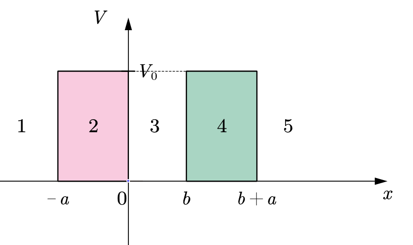
Figure 1. Sketch of the symmetric double barrier.

There are five regions in Figure 1. Region 2 and 4 are assumed to be two same potential barriers, whose height is \( {V_{0}} \) . The potential at region 3 is supposed to be zero which is the same as the potential of the region 1 and 5, since the system is the symmetric double barrier. The article supposes that the particle incidence occurs in Section 1 and the particle emission occurs in the Region 5. Besides, the energy of the particle always satisfies \( {E \lt V_{0}} \) By using the Schrödinger equation in the five regions, the wave functions in these five sections are deduced as

\( ψ(x)=\begin{cases} \begin{array}{c} A{e^{i{k_{1}}x}} +B{e^{-i{k_{1}}x}} , x in 1 \\ C{e^{{k_{2}}x}} +D{e^{-{k_{2}}x}}, x in 2 \\ F{e^{i{k_{1}}x}} +G{e^{-i{k_{1}}x}}, x in 3 \\ H{e^{{k_{2}}x}} +I{e^{-{k_{2}}x}},x in 4 \\ J{e^{i{k_{1}}x}},x in 5 \end{array} \end{cases} .\ \ \ (1) \)

The existed coefficients which describe the amplitudes of five functions are to be determined by combining the boundary conditions. Wave vectors \( {k_{1}} \) and \( {k_{2}} \) both satisfy the following equations \( {{k_{1}}^{2}}=\frac{2mE}{{ℏ^{2}}} \) and \( k_{2}^{2}=\frac{2m({V_{0}}-E)}{{ℏ^{2}}} \) ,where \( m \) is the mass of the particle. In addition, the boundary conditions are

\( \begin{cases} \begin{array}{c} A{e^{-i{k_{1}}a}}+B{e^{i{k_{1}}a}}=C{e^{-{k_{2}}a}}+D{e^{{k_{2}}a}} \\ C+D=F+G \\ F{e^{i{k_{1}}b}}+G{e^{-i{k_{1}}b}}=H{e^{{k_{2}}b}}+I{e^{-{k_{2}}b}} \\ H{e^{{k_{2}}(a+b)}}+I{e^{-{k_{2}}(a+b)}}=J{e^{i{k_{1}}(a+b)}} \\ i{k_{1}}A{e^{-i{k_{1}}a}}-i{k_{1}}B{e^{i{k_{1}}a}}={k_{2}}C{e^{-{k_{2}}a}}-{k_{2}}D{e^{{k_{2}}a}} \\ {k_{2}}C-{k_{2}}D=i{k_{1}}F-i{k_{1}}G \\ i{k_{1}}F{e^{i{k_{1}}b}}-i{k_{1}}G{e^{-i{k_{1}}b}}={k_{2}}H{e^{{k_{2}}b}}-{k_{2}}I{e^{-{k_{2}}b}} \\ {k_{2}}H{e^{{k_{2}}(a+b)}}-{k_{2}}I{e^{-{k_{2}}(a+b)}}=i{k_{1}}J{e^{i{k_{1}}(a+b)}} \end{array} \end{cases}\ \ \ (2) \)

To simplify the calculation, the article supposes that \( A=1 \) . Thus, TC should be

\( T=J\cdot {J^{*}}=\frac{{{C_{3}}^{2}}}{{{C_{1}}^{2}}+{{C_{2}}^{2}}}.\ \ \ (3) \)

The expression of \( {C_{1}} \) , \( {C_{2}} \) , and \( {C_{3}} \) satisfy the following equations

\( \begin{cases} \begin{array}{c} {C_{1}}=4{γ^{2}}cosh{(2a{k_{2}})}cos{(b{k_{1}})}-2αγsinh{(2a{k_{2}})}sin{(b{k_{1}})} \\ {C_{2}}={α^{2}}cosh{(2a{k_{2}})}sin{(b{k_{1}})}-2αγsinh{(2a{k_{2}})}cos{(b{k_{1}})}-{β^{2}}sin{(b{k_{1}})} \\ {C_{3}}=4{γ^{2}} \end{array} \end{cases}\ \ \ (4) \)

where \( α \) , \( β \) , and \( γ \) satisfy the restrictions

\( \begin{cases} \begin{array}{c} α={{k_{1}}^{2}}-{{k_{2}}^{2}} \\ β={{k_{1}}^{2}}+{{k_{2}}^{2}} \\ γ={k_{1}}{k_{2}} \end{array} .\end{cases}\ \ \ (5) \)

After deducing the exact expression of TC, the article will plot the relation between TC and the geometric parameters of the barrier and the energy of the incident particle.

The first is the impact of the change of the width \( a(nm) \) of the barriers. Figure 2 is the relation between TC and the energy corresponding to different values of \( a \) . Besides, the distance and the height of the barriers are fixed as \( b=2nm \) , \( {V_{0}}=1eV \) . By changing the width of the barriers, TC is changing rapidly as well. When the width of the barriers increases, the peak of TC is more obvious, especially when \( a=2nm \) in Figure 2.

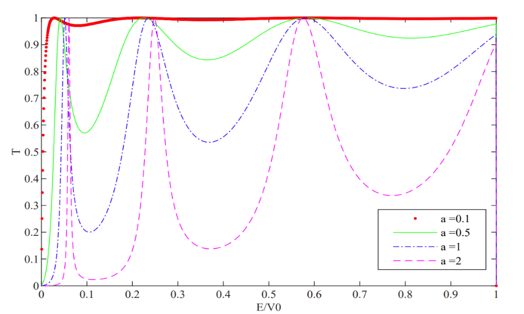
Figure 2. The effect of \( a(nm) \) on the transmission coefficient \( T \) .

The second is the impact of the change of the distance \( b(nm) \) of the barrier. Figure 3 is the relation between TC and the energy corresponding to different values of \( b \) . The width and the height of the barriers are fixed as \( a=0.1nm \) , \( {V_{0}}=1eV \) . Similarly, when the distance of the barriers increases, the peak of TC is more obvious. However, what is different with Figure 2 is that the peak of TC increases with the distance of the barriers rising.

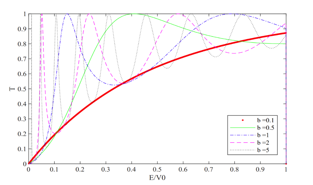
Figure 3. The effect of \( b(nm) \) on the transmission coefficient \( T \) .

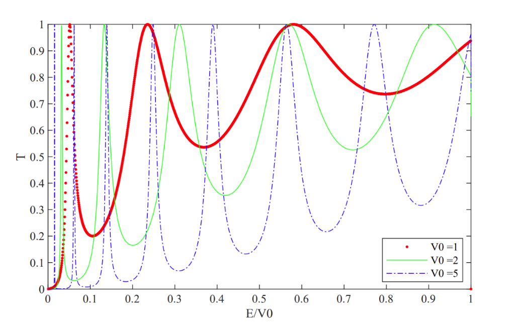
Figure 4. The effect of \( {V_{0}}(eV) \) on the transmission coefficient \( T \) .

The third is the impact of the change of the height \( {V_{0}}(eV) \) of the barriers. Figure 4 is the relation between TC and the energy corresponding to different values of \( {V_{0}} \) . The width and the distance of the barriers are \( a=0.1nm \) , \( b=2nm \) . Equally, when the height of the barriers increases, the peak of TC is more obvious as well. Besides, when \( {V_{0}} \) is big enough, like \( {V_{0}}=20eV \) , the energy corresponding to the first four peaks is \( {E_{1}}=0.00655eV \) , \( {E_{2}}=0.02625eV \) , \( {E_{3}}=0.05935eV \) , \( {E_{4}}=0.10605eV \) . The ratio of these four values almost satisfies 1:4:9:16, which means that there may exist the eigenenergy like the infinite potential well [7]. In addition, the condition of resonant tunneling can be obtained by solving \( T=1 \) .

2.2. Asymmetric double barrier

To plot the relation between TC of asymmetric double barrier and the energy of the particle, the article makes one of the models firstly, as shown in Figure 5, where \( {V_{1}} \) and \( {V_{2}} \) represent the height of the barriers.

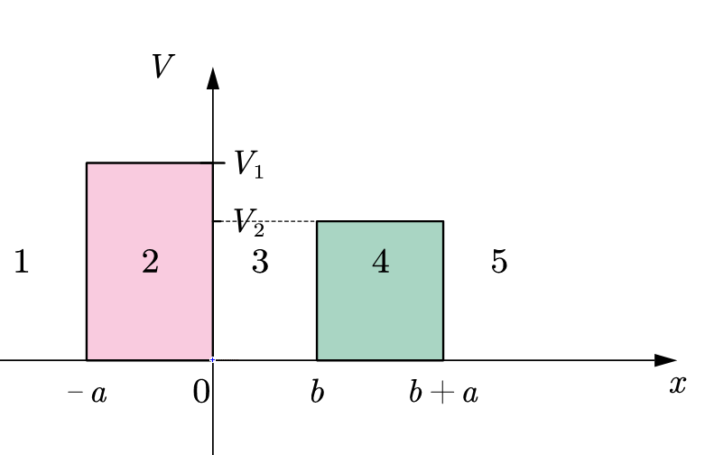
Figure 5. Sketch of the asymmetric double barrier.

Similarly, in the condition: \( {E \lt V_{2}} \lt {V_{1}} \) , the wave functions of these five regions are given by solving the Schrödinger equation in five regions

\( ψ(x)=\begin{cases} \begin{array}{c} {A^{ \prime }}{e^{i{k_{1}}x}} +{B^{ \prime }}{e^{-i{k_{1}}x}} , x in 1 \\ {C^{ \prime }}{e^{{k_{2}}x}} +{{D^{ \prime }}e^{-{k_{2}}x}}, x in 2 \\ {F^{ \prime }}{e^{i{k_{1}}x}} +{G^{ \prime }}{e^{-i{k_{1}}x}}, x in 3\ \ \ \ \ \ \\ {{H^{ \prime }}e^{{k_{3}}x}} +{I^{ \prime }}{e^{-{k_{3}}x}},x in 4 \\ {J^{ \prime }}{e^{i{k_{1}}x}},x in 5 \end{array} \end{cases}\ \ \ (6) \)

These existed coefficients which are to be determined by using the boundary conditions as well. In addition, wave vectors \( {k_{1}} ,{k_{2}}, \) and \( {k_{3}} \) which are existed in the equation all satisfy the following equations: \( {{k_{1}}^{2}}=2mE/{ℏ^{2}} \) , \( k_{2}^{2}=2m({V_{1}}-E)/{ℏ^{2}} \) and \( k_{3}^{2}={2m({V_{2}}-E)/ℏ^{2}} \)

To find TC, the boundary condition in this model should be set. In fact, the boundary condition can be similarly confirmed as Eq (2):

\( \begin{cases} \begin{array}{c} A{ \prime e^{-i{k_{1}}a}}+{B^{ \prime {e^{i{k_{1}}a}}}}=C{ \prime e^{-{k_{2}}a}}+{D^{ \prime {e^{{k_{2}}a}}}} \\ {C^{ \prime }}+{D^{ \prime }}={F^{ \prime }}+{G^{ \prime }} \\ {F^{ \prime {e^{i{k_{1}}b}}}}+{G^{ \prime {e^{-i{k_{1}}b}}}}={H^{ \prime {e^{{k_{3}}b}}}}+I{ \prime e^{-{k_{3}}b}} \\ {H^{ \prime {e^{{k_{3}}(a+b)}}}}+{I^{ \prime {e^{-{k_{3}}(a+b)}}}}=J{ \prime e^{i{k_{1}}(a+b)}} \\ i{k_{1}}{A^{ \prime {e^{-i{k_{1}}a}}}}-i{k_{1}}{B^{ \prime {e^{i{k_{1}}a}}}}={k_{2}}{C^{ \prime {e^{-{k_{2}}a}}}}-{k_{2}}{D^{ \prime {e^{{k_{2}}a}}}} \\ {k_{2}}{C^{ \prime }}-{k_{2}}{D^{ \prime }}=i{k_{1}}{F^{ \prime }}-i{k_{1}}{G^{ \prime }} \\ i{k_{1}}F{ \prime e^{i{k_{1}}b}}-i{k_{1}}{G^{ \prime {e^{-i{k_{1}}b}}}}={k_{3}}H{ \prime e^{{k_{3}}b}}-{k_{3}}{I^{ \prime {e^{-{k_{3}}b}}}} \\ {k_{3}}{H^{ \prime {e^{{k_{3}}(a+b)}}}}-{k_{3}}{I^{ \prime {e^{-{k_{3}}(a+b)}}}}=i{k_{1}}{J^{ \prime {e^{i{k_{1}}(a+b)}}}} \end{array} \end{cases}.\ \ \ (7) \)

Here, the TC can be derived from Eq. (7). After obtaining TC, the effects of different parameters can be easily plotted.

Figure 6 \( {({V_{1}}=1eV,V_{2}}=0.8eV,b=2nm) \) is the figure which describes the impact of the width \( a(nm) \) . The general image is similar to the previous one which also describes the impact of the width in the symmetric double barrier. What is different from the former one is the peak of TC cannot equal to 1. Besides, when \( E→{V_{2}} \) , TC will decrease instead of being closed to 1.

In fact, Figure 7 ( \( {V_{1}}=1eV, a=0.1 nm ,b=2nm) \) shows that when \( {V_{2}} \) increases, the peak of TC is similar to Fig.2. When the initial condition \( { E \lt V_{2}} \lt {V_{1}} \) have changed into \( { E \lt V_{1}} \lt {V_{2}} \) , TC will be sometime greater than 1, the figure will be totally different from Figure 7. However, there also exists some similar peaks as the symmetric situation. When the energy equals to some certain values, TC will reach the peak. This situation will be more obvious as the width increasing, since, in Figure 6, the peaks are becoming separated as width rises.

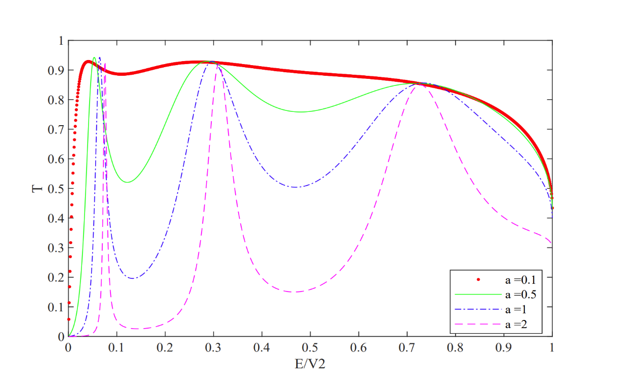
Figure 6. The effect of \( a(nm) \) on the transmission coefficient \( T \) .

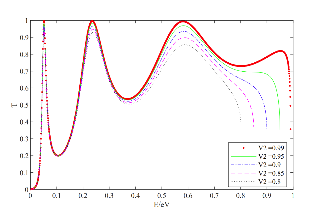
Figure 7. The effect of \( {V_{2}}(eV) \) on the transmission coefficient \( T \) .

3. Application

After discussing one-dimensional double barrier including symmetric and asymmetric double barrier, the article has extended the discussion to the one-dimensional periodic barrier. Similarly, when considering periodic barrier, one of the situations is repeating symmetric double barrier in one-dimension. Another situation is repeating asymmetric double barrier. In fact, the first situation has already discussed by many researchers by using transition matrix [8]. In fact, the kernel of transition matrix equals to the method of solving the Schrödinger equation. The computation of transition matrix is more compatible with the computing method of computers. It is a convenient way to get TC by using the computer.

In addition, the relation between TC and the energy is similar to Figure 2 [9]. However, the difference between them is the values corresponding to the peaks are more than the symmetric double barrier. Besides, when the energy is the value which between two multi-peaks, TC will be zero, which means if the energy of the particle is certain energy between the peaks, the particle will be reflected and found only in region 1 in Fig.1. On the contrary, when the energy of the particle is the value of multi-peaks, the particle will be transmitted and found in region 5 in Figure 1. Based on this property, band structure theory was built which can describe the principle of the semiconductor. Band structure theory is also a significant theory in Solid States Physics and can help researchers comprehend some molecules deeply like beta-Ga₂O₃ [10].

4. Conclusion

In conclusion, the TC of double barrier including symmetric and asymmetric barrier has the similarity to the eigenenergy of the potential barrier. When the energy equals to certain energy, the TC will reach the peak. Based on this property, many devices can be built. In addition, some parameters can affect the TC of symmetric double barrier, such as the barrier width, height and the distance. These parameters all have similar effects on TC. When the parameters rise, the peaks of TC will be more obvious and separated. On the other hand, the condition of resonant tunnelling is also given in the article. As for the asymmetric double barrier, when the height of the barrier becomes to the same, the TC will be equal to the symmetric situation, which proves the accuracy of the exact expression of TC. Besides, TC of the asymmetric double barrier is similar to TC of symmetric double barrier. Based on these properties, the main contribution of this article will help the tyro and researchers apprehend and analyse the relevant devices. The method used in this paper still has the difficulties of complicated calculation and a simpler method should be found for future research such as transition matrix.

References

[1]. Preskill, J. (2018). Quantum Computing in the NISQ era and Beyond, Quantum, 2, 79.
[2]. Zhang Z. H, et al. (2023). Toward High-Peak-to-Valley-Ratio Graphene Resonant Tunneling Diodes. Nano Letters, 23(17), 8132-39.
[3]. Ke C. Q, and Ding Y. M. (2015). Research of Transmission Coefficient of Potential Barrier Penetration Based on Matlab. Physics And Engineering, 25(01), 76-77+79.
[4]. Sacchetti A. (2023). Tunnel Effect and Analysis of the Survival Amplitude in the Nonlinear Winter’s Model. Annals of Physics, 457, 169434.
[5]. Abdullaev F. K, Galimzyanov R. M. and Shermakhmatov A. M. (2023). Effects of Quantum Fluctuations on Macroscopic Quantum Tunneling and Self-Trapping of a BEC in a Double-Well Trap. Journal of Physics B-Atomic Molecular and Optical Physics, 56(16).
[6]. Li C Z, Lin XC. (2005). Numerov Algorithm for Tunneling. Journal of Xidian University, 32(01), 12-15.
[7]. Xia W J, Zhang L. (2015). Research on Infinite Potential Well in Quantum Mechanics Teaching. College Physics, 34(02), 35-40.
[8]. Gong J P. (2012). One-Dimensional Double Barrier Scattering Problem. Journal of Jinzhong University, 29(03),19-24.
[9]. Luo M, Yang S B. (2012). Calculation of Resonant Transmission Coefficient for Multi-Barrier Structure. Journal of Nanjing Normal University (Natural Science Edition), 35(02), 50-55.
[10]. Peelaers H, Van de walle C. (2015). Brillouin zone and band structure of beta-Ga2O3. Physica Status Solidi B-Basic Solid-State Physics, 252(4), 828-32.
Cite this article
Li,J. (2023). The discussion of the transmission coefficient of one-dimensional double barrier. Theoretical and Natural Science,25,166-172.
Data availability
The datasets used and/or analyzed during the current study will be available from the authors upon reasonable request.
Disclaimer/Publisher's Note
The statements, opinions and data contained in all publications are solely those of the individual author(s) and contributor(s) and not of EWA Publishing and/or the editor(s). EWA Publishing and/or the editor(s) disclaim responsibility for any injury to people or property resulting from any ideas, methods, instructions or products referred to in the content.
About volume
Volume title: Proceedings of the 3rd International Conference on Computing Innovation and Applied Physics
© 2024 by the author(s). Licensee EWA Publishing, Oxford, UK. This article is an open access article distributed under the terms and
conditions of the Creative Commons Attribution (CC BY) license. Authors who
publish this series agree to the following terms:
1. Authors retain copyright and grant the series right of first publication with the work simultaneously licensed under a Creative Commons
Attribution License that allows others to share the work with an acknowledgment of the work's authorship and initial publication in this
series.
2. Authors are able to enter into separate, additional contractual arrangements for the non-exclusive distribution of the series's published
version of the work (e.g., post it to an institutional repository or publish it in a book), with an acknowledgment of its initial
publication in this series.
3. Authors are permitted and encouraged to post their work online (e.g., in institutional repositories or on their website) prior to and
during the submission process, as it can lead to productive exchanges, as well as earlier and greater citation of published work (See
Open access policy for details).