1. Introduction

Bitcoin is a Peer-to-peer (P2P) form of virtual currency that is generated through large-scale computing based on certain algorithms. Users trade through Bitcoin wallets and addresses. Due to the advancement of modern technology, the trading of Bitcoin has become more widespread and frequent. People profit from the price fluctuations of Bitcoin by buying and selling. Due to the similarity between its trading and stocks, the prediction of Bitcoin prices and returns has become a research topic.

The traditional solution to price and return prediction is to use multiple specific statistical models and evaluate a series of technical indicators to assess the precision. However, traditional methods often overlook the intricate and non-linear associations of data, making the prediction results sometimes lack reference value.

In recent years, deep learning models have developed rapidly, among which the Long Short Term Memory (LSTM) can better capture permanent dependencies and nonlinear models in time series data, and has better adaptability in prediction problems.

On this basis, this paper uses the LSTM to forecast the price and return of Bitcoin trading by comparing past data of Bitcoin trading. By training this model, it can learn the patterns and trends in the Bitcoin trading market, thereby achieving prediction of future Bitcoin trading returns. Due to its complex network structure and attention to time series data, the LSTM model enhances the precision of forecasting and has stronger real-time prediction ability and better assistance in investment decision-making. Through such predictions, investors and researchers can more accurately grasp the future market trends and help them make more informed investment decisions.

2. Literature Review

In recent years, the Bitcoin trading market has received more attention, so many researchers have conducted in-depth research on it. In 2017, H Jang and J Lee used the Bayesian Neural Network (BNN) to examine the time series for Bitcoin transaction data [1]. They also selected the most pertinent attributes of Bitcoin transactions extracted from the blockchain data. This resulted in an improved performance in prediction. In 2018, S Velankar et al. were the first to explore Bitcoin market trends and research the best features that influence Bitcoin prices and constructing a dataset containing daily transaction data over five years [2]. Various features extracted from Bitcoin prices and payments on the blockchain are used with existing information to predict daily price changes with the highest possible accuracy. In 2019, S Ji et al. used various neural network models to study Bitcoin, including not only stand-alone neural networks, but also combinations of these networks [3]. In 2020, Z Chen et al. looked at using machine learning techniques to predict Bitcoin prices at different frequencies [4]. They begin by categorising Bitcoin prices into the following two categories: daily prices and high-frequency prices. The daily price of Bitcoin is predicted by focusing on specific high-dimensional features, such as assets on the blockchain, trading networks, and current market conditions, and the price of Bitcoin within a five-minute range is predicted by extracting features from information obtained from the cryptocurrency's exchanges.

3. Methodology

The experimental dataset in this paper is from Kaggle, which includes Bitcoin trading data from 2012 to 2021. In this paper, firstly, the transaction data of Bitcoin is preprocessed, which includes normalization operations to control the data difference within a small range. Then the data is inputted into the LSTM (Autoregressive Integrated Moving Average (ARIMA) and eXtreme Gradient Boosting (XGBoost) as a comparison) and trains it. Finally, use the trained model for prediction. The final prediction result has three evaluation indicators: Mean Square Error (MSE), Root Mean Square Error (RMSE), Mean Absolute Error (MAE).

3.1. Bitcoin transaction dataset with timestamps

The dataset, referred to as 'Bitcoin Historical Data', is sourced from Kaggle. The dataset includes Bitcoin data provided by a specific exchange from January 2012 to March 2021. It provides up-to-the-minute reporting on the OHLC (open high low close), volume, weighted price, etc. Timestamps are given in Unix time. Those timestamps containing no transactions or activity are presented with NaNs filling their data fields.

3.2. MinMaxScaler normalization

Data normalization involves limiting the range of data that requires processing via a specific algorithm. This aids subsequent data processing and speeds up program execution. The principal function of normalization is to statistically unify a sample distribution. Normalization places the values of the data in the interval 0 to 1. This method is a probability distribution often used in statistics. Normalization places data values within a certain interval. This method is a coordinate distribution often used in statistics. MinMaxScaler normalizes a set of data so that its values range from 0 to 1, in order to eliminate factors that cause significant differences in values between different features in different results. The formula is as follows.

\( {x^{*}}=\frac{x-min{(x)}}{max{(x)}-min{(x)}} \) (1)

In formula 1, the current value \( x \) subtracted by the minimum value \( min{(x)} \) in the dataset is represented by the numerator, while the denominator represents the disparity between the two end values of the interval in the dataset.

3.3. LSTM structure

LSTM is a specific Recurrent Neural Network (RNN) [5]. When RNN receives a long time series, the transfer of information between two distant time steps becomes a difficult problem to solve. while LSTM can learn long-term dependent information, better connect with context, and solve the problem of insufficient short-term memory in RNN.

The three gates together form the LSTM. Through the functions of these three gates, information is controlled and transmitted. As shown in figure 1.

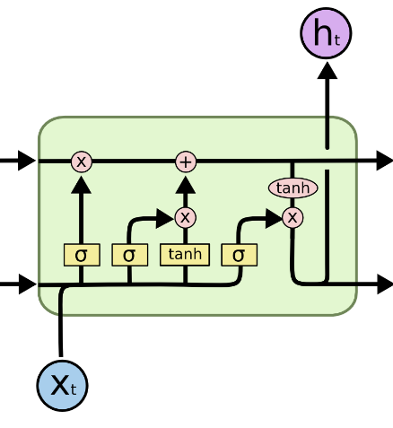
Figure 1. LSTM unit

3.3.1. Gate. LSTM controls the state of cells through gates, allowing cells to forget or add memories. The gate's structure comprises a sigmoid layer that multiplies the previous moment's cell state. The output value from the sigmoid layer ranges from 0 to 1, which can be used as a gate control signal. 0 represents memory forgetting, and 1 represents memory addition.

3.3.2. Forget gate. The object of the forgetting gate is the cell state, and its function is to regulate the information in the cell state, forget it or add it. The specific formula is as follows.

\( {f_{t}}=σ({W_{f}}\cdot [{h_{t-1}},{x_{t}}]+{b_{f}}) \) (2)

In formula 2, first get the input \( {x_{t}} \) , then get the hidden state \( {h_{t-1}} \) , and splice the two together, that is, \( [{h_{t-1}},{x_{t}}] \) . Multiply the result obtained in the previous step with the weight matrix \( {W_{f}} \) and add the bias \( {b_{f}} \) . Finally, \( {f_{t}} \) is obtained by sigmoid activation function \( σ \) .

The gate value \( {f_{t}} \) is a crucial aspect through which each tensor passes. As the cell state of the preceding layer enters the oblivion gate, the corresponding gate value would determine the extent of information that is lost. The oblivion gate value is computed from \( {x_{t}} \) and \( {h_{t-1}} \) . This formula means that the cells in the upper layer selectively discard part of the information and selectively retain part of the information. The amount of this information depends on the previously mentioned input \( {x_{t}} \) and hidden state \( {h_{t-1}} \) .

3.3.3. Input gate. The target of the input gate is also the cell state. Its function is to determine what information will be in storage, that is, the cell state selectively adds memory. The input gate is composed of two components. The specific formula is as follows.

\( {i_{t}}=σ({W_{i}}\cdot [{h_{t-1}},{x_{t}}]+{b_{i}}) \) (3)

\( \widetilde{{C_{t}}}=Tanh({W_{c}}\cdot [{h_{t-1}},{x_{t}}]+{b_{C}}) \) (4)

In formula 3, similar to formula 2, first get the input \( {x_{t}} \) , then get the hidden state \( {h_{t-1}} \) , and splice the two together, that is, \( [{h_{t-1}},{x_{t}}] \) . Multiply the result obtained in the previous step with the weight matrix \( {W_{i}} \) and add the bias \( {b_{i}} \) . Finally, \( {i_{t}} \) is obtained by sigmoid activation function \( σ \) .

This formula generates the input gate value and closely resembles the forget gate formula. But the distinction lies in the target that will be applied at a later stage. This formula means that after the information is entered, part of it is retained and part needs to be filtered out.

In formula 4, similar to formula 2, first get the input \( {x_{t}} \) , then get the hidden state \( {h_{t-1}} \) , and splice the two together, that is, \( [{h_{t-1}},{x_{t}}] \) . Multiply the result obtained in the previous step with the weight matrix \( {W_{c}} \) and add the bias \( {b_{c}} \) . Finally, \( \widetilde{{C_{t}}} \) is obtained by Tanh activation function.

Similar to the way cells are calculated inside RNN, this formula is used for cell state updates. Multiply the cell state \( {C_{t-1}} \) by the output of the forget gate; then multiply the unupdated cell state \( {C_{t}} \) by the output of the input gate. Add these two results to obtain the updated cell state \( {C_{t}} \) , which is used as the input.

3.3.4. Output gate. The function of the output gate is to determine what is the final output. The output gate also contains two parts. The specific formula is as follows.

\( {o_{t}}=σ({W_{o}}\cdot [{h_{t-1}},{x_{t}}]+{b_{o}}) \) (5)

\( {h_{t}}={o_{t}}*Tanh({C_{t}}) \) (6)

In formula 5, similar to formula 2, first get the input \( {x_{t}} \) , then get the hidden state \( {h_{t-1}} \) , and splice the two together, that is, \( [{h_{t-1}},{x_{t}}] \) . Multiply the result obtained in the previous step with the weight matrix \( {W_{o}} \) and add the bias \( {b_{o}} \) . Finally, \( {o_{t}} \) is obtained by sigmoid activation function \( σ \) .

This formula calculates the output gate value and follows the same calculation method as the forget and input gates.

In formula 6, the new cell state \( {C_{t}} \) is transmitted to the Tanh activation function. The result obtained is cross-multiplied with the result \( {o_{t}} \) obtained in formula 5 to obtain \( {h_{t}} \) .

This formula calculates the amount of information to be conveyed by the hidden state. The hidden state that conveys the information is then transmitted to the next time step as the current cell output.

3.4. ARIMA model in prediction

The ARIMA Model [6], is composed of three key components: Auto Regressive (AR), Integrated (I), Moving Average (MA).

The aim of the ARIMA is to predict future data using the historical information it has gathered. This model learns the mode of the series in the data by studying the correlation and difference of the data itself, which will be used for data prediction.

AR is used for parts of time series data with autoregressive characteristics. It focuses on observed values in past periods and analyzes the impact of these values on current values.

I is used to make non-stationary time series stationary and eliminate trend and seasonal factors in the time series through first-order or second-order difference processing.

MA is used to process the moving average part of the time series. It focuses on past prediction errors and analyzes the impact of these errors on current values.

The three parts combine and work so that the ARIMA model not only learns the changing trends of the data but also handle data with temporary, sudden changes, or noisy data.

3.5. XGBoost model in prediction

XGBoost trains one tree and then trains the next tree to predict the gap between it and the real distribution [7]. It makes up for the gap through continuous training and finally uses a combination of trees to simulate the real distribution.

In XGBoost, trees are units that increase or decrease in number and are used to fit the residuals of previous predictions by learning functions. Each time a tree is added to the model, the above process is repeated. This is the core algorithm of the model. The tree is formed through feature splitting. When the model completes training, that is, after repeating the above process several times and obtaining several such trees, it proceeds to predict the score of the sample. For each different sample, each tree will drop a leaf with a specific score, determined by the sample characteristics. The prediction score of the sample is the sum of these leaf scores.

The purpose of this form is to minimize the gap between the real and the predicted and make the model have strong generalization ability in prediction problems.

3.6. Evaluation under the MSE RMSE MAE indicator

This paper uses four evaluation indicators, The specific formula and explanation are as follows.

\( MSE=\frac{1}{n}\sum _{i=1}^{n}{(\hat{{y_{i}}}-{y_{i}})^{2}} \) (7)

In formula 7, for every instance, determine the difference between the estimated \( \hat{{y_{i}}} \) and the real \( {y_{i}} \) , then subsequently apply the square of this deviation. Then sum all the differences and divide by the number of observations to get the mean squared error, or MSE.

MSE is a prevalent measure that quantifies the deviation between the predictions and the observed data. It is extensively utilized in assessing the model's accuracy in fitting the given data [8].

\( RMSE=\sqrt[]{\frac{1}{n}\sum _{i=1}^{n}{(\hat{{y_{i}}}-{y_{i}})^{2}}} \) (8)

In formula 8, for every instance, determine the difference between the estimated \( \hat{{y_{i}}} \) and the real \( {y_{i}} \) , then subsequently apply the square of this deviation. Then sum all the differences and divide by the total number of observations to get MSE, and finally take the square root of MSE, or RMSE.

RMSE is a prevalent method of assessing the disparity between a model's forecasts and genuine observations. It is utilised to assess the model's suitability to the provided data. RMSE is determined by averaging of the squared deviation between the predicted and observed, then taking the square root.

\( MAE=\frac{1}{n}\sum _{i=1}^{n}|\hat{{y_{i}}}-{y_{i}}| \) (9)

In formula 9, for each observation, calculate the absolute value of the deviation between the predicted value \( \hat{{y_{i}}} \) and the actual observation \( {y_{i}} \) , sum all the differences and divide by the number of observations to get MAE.

MAE is a widely-employed measurement that assesses the extent of variance between model forecasts and observed results. Its function is to evaluate the accuracy of a model's agreeability with provided data [9]. MAE is computed by averaging the absolute discrepancies between anticipated and observed values.

4. Result

The results of the experiment are displayed in the following table. All results retain three significant figures.

Table 1. Experimental result

4.1. Performance Comparison on LSTM with ARIMA and XGboost

Observing the data in table 1, it can see that for the Bitcoin return issue, the LSTM model exhibits better performance in comparison to the ARIMA and XGBoost models on the three indicators of MSE, RMSE, and MAE. There is almost no difference in performance between the ARIMA and XGBoost models, but the LSTM model due to the complexity of its network structure, the running time longer than the other two models.

4.2. Further Discussion about Bitcoin Prediction

Based on the existing models at the time, previous researchers conducted in-depth research on the Bitcoin prediction problem and obtained accurate and convincing research results. However, in recent years, deep learning models have developed rapidly, and models have been continuously updated and improved. Especially in time series prediction models, many models with excellent performance have emerged, such as Neural Basis Expansion Analysis for Interpretable Time Series Forecasting (N-BEATS) and Deep Auto Regressive (DeepAR) [10,11]. They all demonstrate strong functionality in different tasks. Bitcoin prediction problems should keep pace with the times, and constantly combine old problems with new models. On the one hand, it can obtain more accurate and convincing results, and on the other hand, it can also promote the update and progress of models for specific problems, making it possible to The field of prediction for similar problems has better prospects for development.

5. Conclusion

This paper draws on previous research on Bitcoin price prediction based on LSTM and then studies the Bitcoin return prediction problem based on the LSTM model. In terms of code, in the price prediction part, the original author's code is retained, while in the return prediction part, the code is completed independently. In terms of data, preprocessing was performed similarly to that of the original author; in terms of models, construction, training, and prediction were completed, and the coding style was consistent with the previous code; in terms of evaluation, three more common evaluation indicators were used. Regarding the controlled experiment, this paper uses two common time series prediction models, ARIMA and XGBoost, to better highlight the advantages and disadvantages of LSTM in this experiment.

Overall, compared to the other two models, the LSTM model performs better on this problem, which is a good result. However, in terms of model complexity, LSTM is more complex than the other two models, so it has a longer running time. Throughout the experiment, due to time constraints, there were few adjustments to parameters, and the performance of each model under different parameters was not obtained, otherwise, this would be a more convincing result.

References

[1]. Jang, H. Lee, J. 2017, An empirical study on modeling and prediction of bitcoin prices with bayesian neural networks based on blockchain information. (Ieee Access, vol. 6), pp. 5427-5437.
[2]. Velankar, S. Valecha S. Maji S. 2018, Bitcoin price prediction using machine learning. (In 2018 20th International Conference on Advanced Communication Technology ICACT, IEEE), pp. 144-147.
[3]. CJi S. Kim J. Im, H. 2019, A comparative study of bitcoin price prediction using deep learning. (Mathematics, vol. 7), no. 10, pp. 898.
[4]. Chen, Z. Li, C. Sun, W. 2020, Bitcoin price prediction using machine learning: An approach to sample dimension engineering, (Journal of Computational and Applied Mathematics, vol. 365), pp. 112395.
[5]. Staudemeyer, R. C. Morris, E. R. (2019). Understanding LSTM--a tutorial into long short-term memory recurrent neural networks. arXiv preprint arXiv:1909.09586.
[6]. Shumway, R H. Stoffer, D S. Shumway, R H. Stoffer, D S. 2017, Time series analysis and its applications: with R examples, (ARIMA models), pp. 75-163.
[7]. Chen, T. He, T. Benesty, M. Khotilovich, V. Tang, Y. Cho, H. 2015, Xgboost: extreme gradient boosting. (R package version , vol. 1), no. 4, pp. 1-4.
[8]. Marmolin, H. 1986, Subjective MSE measures. (IEEE transactions on systems, man, and cybernetics, vol. 16), no. 3, pp. 486-489.
[9]. Chai, T. Draxler, R R. 2014, Root mean square error (RMSE) or mean absolute error (MAE). (Geoscientific model development discussions, vol. 7), no. 1, pp. 1525-1534.
[10]. Sbrana, A., Rossi, A. L. D. Naldi, M. C. (2020, December). N-BEATS-RNN: deep learning for time series forecasting. In 2020 19th IEEE International Conference on Machine Learning and Applications (ICMLA), pp. 765-768.
[11]. Salinas, D. Flunkert, V. Gasthaus, J. Januschowski, T. 2020. DeepAR: Probabilistic forecasting with autoregressive recurrent networks. (International Journal of Forecasting, vol. 36), no. 3, pp. 1181-1191.
Cite this article
Yang,R. (2023). Bitcoin price and return prediction based on LSTM. Theoretical and Natural Science,26,74-80.
Data availability
The datasets used and/or analyzed during the current study will be available from the authors upon reasonable request.
Disclaimer/Publisher's Note
The statements, opinions and data contained in all publications are solely those of the individual author(s) and contributor(s) and not of EWA Publishing and/or the editor(s). EWA Publishing and/or the editor(s) disclaim responsibility for any injury to people or property resulting from any ideas, methods, instructions or products referred to in the content.
About volume
Volume title: Proceedings of the 3rd International Conference on Computing Innovation and Applied Physics
© 2024 by the author(s). Licensee EWA Publishing, Oxford, UK. This article is an open access article distributed under the terms and
conditions of the Creative Commons Attribution (CC BY) license. Authors who
publish this series agree to the following terms:
1. Authors retain copyright and grant the series right of first publication with the work simultaneously licensed under a Creative Commons
Attribution License that allows others to share the work with an acknowledgment of the work's authorship and initial publication in this
series.
2. Authors are able to enter into separate, additional contractual arrangements for the non-exclusive distribution of the series's published
version of the work (e.g., post it to an institutional repository or publish it in a book), with an acknowledgment of its initial
publication in this series.
3. Authors are permitted and encouraged to post their work online (e.g., in institutional repositories or on their website) prior to and
during the submission process, as it can lead to productive exchanges, as well as earlier and greater citation of published work (See
Open access policy for details).