1. Introduction

Control systems constitute a pivotal component in modern engineering and technology, dictating the performance and stability of numerous critical applications. Whether in the automation of manufacturing lines, autonomous vehicles in transportation, or precise control systems in medical devices, the role of control systems cannot be understated. Currently, Proportional Integral Derivative (PID) controllers, a form of feedback control, dominate the field, accounting for over 90% of all control loops [1]. However, most controllers employed in industrial settings frequently encounter the risk of system instability, necessitating the establishment of robust feedback systems [2]. A classical approach is the Ziegler-Nichols method, which aims to maintain system stability by tuning the balance between regulation (disturbance suppression) and tracking behavior [3]. Nevertheless, the effectiveness of this method is less than ideal in scenarios with significant noise, frequent setpoint changes, or systems characterized by substantial time delays [2]. Against this backdrop, this paper delves into an in-depth exploration of two common control strategies: proportional feedback control (P control) and integral control (PI control). The focus of this research lies in their application and performance analysis within two distinct yet interconnected domains. Specifically, the author investigates the application of P control in DC motors and the utilization of PI control in speed control. Methodology encompasses both simulation modelling and practical analysis, employing the Tinkercad and Octave tools for intuitive implementation and evaluation of these control strategies. The influence of various control parameters on system responses, with a particular emphasis on step responses and steady-state performance, is also examined. The results of this research are expected to contribute to the enhancement of control system design and performance, thereby propelling technological advancement and innovation across various application domains.

2. Literature review

Shafiei et al. and Anon have optimized methods based on parameter space techniques for analyzing stability regions, emphasizing the role of gain and phase margin in parameter space [2][4]. These stability regions provide sets of controller parameters that ensure a stable closed-loop system. Through the analysis of stability regions, studies have achieved promising results [5-7]. The former relies on the Hermite-Bieler theorem, while the latter two are grounded in complex polynomial calculations. However, practical PID controller design often encounters numerous challenges. It extends beyond the application of classical methods to enhance system stability in more complex systems [3][8]. Several factors must be considered, including the need for controllers to adhere to design specifications, reliance on available/accessible process knowledge, and constraints imposed by computational capabilities and resources available for design [1]. Researchers have yielded results pertaining to several different design procedures characterized by distinct objectives and complexities [9-10].

Recent research in PI control has revealed several notable trends and advancements. Firstly, some studies are focusing on the adaptive adjustment of PI controller parameters to address uncertainties and variations within systems. For instance, the method utilizes fuzzy logic techniques to optimize PI parameters, enhancing the performance of hydrogen pressure control [11]. This approach combines engineering expertise and knowledge, improving the control system's responsiveness to dynamic changes. Secondly, researchers are striving to integrate PI control with other control strategies to enhance system responsiveness and performance. As mentioned in Li et al, a charging strategy employing PI control in conjunction with a high-dimensional nonlinear dynamic model and Ensemble Transform Kalman Filter (ETKF) has been developed for fast charging [12]. This approach not only increases charging speed but also reduces computational costs. Finally, there is a growing focus on further studying and understanding the convergence mechanisms of PI control. It is noted that the convergence of saturated PI control is demonstrated for the first time using an optimization solver and primal-dual neural networks [13]. This method enhances the understanding of PI control principles while improving control efficiency. Researchers are dedicated to enhancing its performance and applicability to meet evolving engineering demands. These studies hold the potential to have a significant impact in fields such as energy systems, battery management, and nonlinear systems.

3. Methods

3.1. Application and analysis of P Control in DC motors

P Control is a straightforward yet effective control strategy that adjusts the control output based on the magnitude of the current error, which is the difference between the actual value and the desired setpoint. When the error is substantial, the P controller generates a large control output to rapidly reduce the error. Conversely, when the error is small, the P controller produces a smaller control output to mitigate control overshoot. P control lacks memory; it solely focuses on the current error and does not consider the past error history.

Tinkercad was used to construct a model of a DC motor, capable of translating input voltage into angular output. The model's transfer function is \( \frac{K}{τs+1}×\frac{1}{s} \) . Within this framework, \( \frac{K}{τs+1} \) represents the transfer function responsible for converting voltage into speed, while \( \frac{1}{s} \) signifies the integrator's transfer function, responsible for translating speed into angle. In the model, the default value of "K" is set to 3, and \( τ \) is defaulted to 0.1 seconds, representing the mechanical time constant of the DC motor. The choice of "K" being set to 3 and "t" being set to 0.1 is often based on practical considerations and the characteristics of the specific system being modeled. These values can vary depending on the specific DC motor and the requirements of the control system being designed. The gain "K" in the transfer function represents the amplification or sensitivity of the system. Setting "K" to 3 might be a reasonable default value if, for instance, it is known from the motor's specifications that a given voltage change of 1 V results in an approximate speed change of 3 units (the specific units depend on the system and motor). A standardized default like "K = 3" makes it easier to compare the results of different control algorithms or scenarios because it provides a common reference point. The time constant " \( τ \) " represents how fast or slow the system responds to changes in the input voltage. A smaller value of " \( τ \) " (0.1 seconds in this case) indicates a relatively fast system response. This might be appropriate if the motor is designed for its rapid reaction to voltage changes. The transfer function of the DC motor itself is \( \frac{3}{0.1{s^{2}}+s} \) .

The schematic diagram of the proportional feedback control circuit is shown in Figure 1:

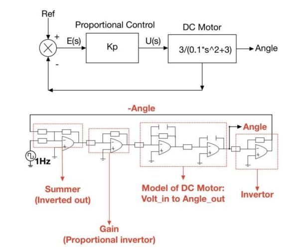
Figure 1. The schematic diagram of the proportional feedback control circuit

The topological structure of the circuit is divided into four parts, from left to right. The first part is the "Summer," which subtracts the 1Hz output of the function generator from the angle. The second part is the gain module. The third part is the model of the DC motor. The fourth part is an inverter responsible for reversing the angle's value. Based on the schematic of the proportional feedback control circuit, the circuit was implemented in Tinkercad, as shown in Figure 2:

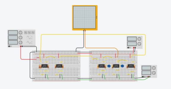
Figure 2. The proportional feedback control circuit in Tinkercad

In Tinkercad, two power supplies were employed to provide a voltage of \( +=15V \) to all operational amplifiers, and an oscilloscope was used to visually display the system's step response. The ratio of resistance values in the gain module's left and right resistors was adjusted to set different values of \( {K_{p}} \) .

When \( {K_{p}} \) is set to 0.5, the ratio of resistance values in the gain module's left and right resistors is 2:1. The oscilloscope's result is depicted in Figure 3:

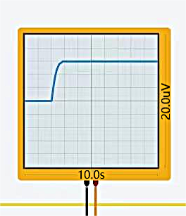
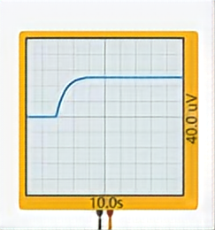
Figure 3. Oscilloscope's result when \( {K_{p}} \) is 0.5 Figure 4. Oscilloscope's result when \( {K_{p}} \) is 1

From the oscilloscope, it can be observed that the system reaches steady-state at approximately 1.8 seconds.

When \( {K_{p}} \) is set to 1, with a ratio of 1:1 for the left and right resistors in the gain module, the oscilloscope's result is shown in Figure 4. Compared to \( {K_{p}} \) being 0.5, the system reaches steady-state faster, in just about 1 second. When \( {K_{p}} \) is set to 3, with a ratio of 1:3 for the left and right resistors in the gain module, the oscilloscope's result is depicted in Figure 5. At this point, the system reaches the target voltage value in very little time, but there are also some overshoots.

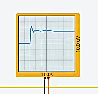
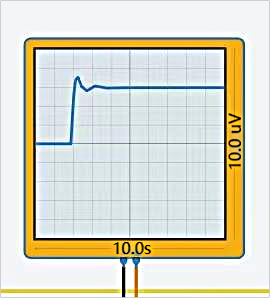
Figure 5. Oscilloscope's result when \( {K_{p}} \) is 3 Figure 6. \( {K_{p}} \) Oscilloscope's result when \( {K_{p}} \) is 5

When \( {K_{p}} \) is set to 5, with a ratio of 1:5 for the left and right resistors in the gain module, the oscilloscope's result is shown in Figure 6. At this setting, compared to being 3, there are more overshoots.

The Root Locus plots for different values are shown in Figure 7, where "Cross" corresponds to \( {K_{p}} \) = 5, "Red" to \( {K_{p}} \) = 3, "Green" to \( {K_{p}} \) = 1, and "Blue" to \( {K_{p}} \) = 0.5.

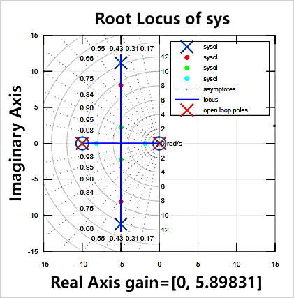
Figure 7. The Root Locus for 4 different values of \( {K_{p}} \)

For \( {K_{p}} \) equal to 0.5, the system's roots lie on the real axis, all with negative values symmetrically around (-5, 0). In this scenario, all poles are located on the real axis and are negative. Since they all lie on the real axis, the damping ratio is 1, indicating a critically damped system. In a critically damped state, the system returns to a steady state as quickly as possible without oscillations. This occurs because a damping ratio of 1 signifies that the oscillation frequency equals the natural frequency but without amplitude growth. Therefore, the system stabilises rapidly without oscillations. For \( {K_{p}} \) values of 1, 3, and 5, the roots are distributed on the imaginary axis with a real part of -5, and the damping ratio gradually decreases as \( {K_{p}} \) increases.

3.2. Proportional-Integral Control in speed control: application and analysis

PI control, an extension of P control, is introduced to address the issue of steady-state error. The integral component of PI control takes into account the historical error to ensure that the system eventually reaches the desired setpoint. While the proportional component still adjusts the control output based on the current error, similar to P control, the integral component considers the sum of past errors to suppress steady-state errors. If there is a steady-state error present in the system, the integral component gradually increases the control output until the error is eliminated. Additionally, the integral component enhances the system's robustness, enabling it to better handle uncertainties and external disturbances.

In the simulation, Octave was employed to model PI control, transforming the input voltage into an output speed. Within the simulation, the transfer function from voltage to speed, denoted as \( \frac{3}{0.1s+1} \) , was utilized. The control module \( C(S) \) had a transfer function represented by \( {K_{p}}+\frac{{K_{I}}}{S} \) , which is given as \( C(S)=\frac{{K_{p}}(S+\frac{{K_{I}}}{{K_{p}}})}{S} \) . The parameters within the control module included \( {K_{p}} \) , which represented the gain module's transfer function, and \( \frac{{K_{I}}}{S} \) , corresponding to the transfer function of the integral module. The values of \( {K_{p}} \) were varied, specifically set to 0.1, 0.3, 0.6, and 1.2, to observe the step response and create the corresponding PZmap.

When \( {K_{p}} \) = 0.1, the corresponding PZmap is shown in Figure 8. Zeros are indicated by red points labeled "O," while poles are represented by red points labeled "X." When \( {K_{p}} \) = 0.3, the corresponding PZmap is displayed in Figure 9.

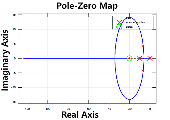
Figure 8. PZmap when \( {K_{p}} \) is 0.1

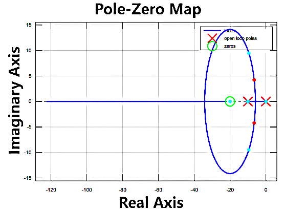
Figure 9. PZmapwhen \( {K_{p}} \) is 0.3

When \( {K_{p}} \) = 0.6, the corresponding PZmap can be seen in Figure 10. When \( {K_{p}} \) = 1.2, the corresponding PZmap is illustrated in Figure 11.

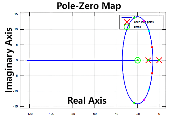
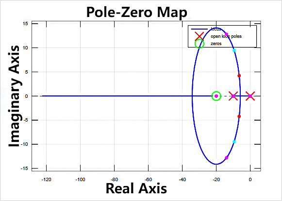
Figure 10. PZmap when \( {K_{p}} \) is 0.6 Figure 11. PZmap when \( {K_{p}} \) is 1.2

The ellipse, as shown in Figure 8-11, with a longer axis along the imaginary axis than the real axis may indicate that the system's frequency response has a resonant frequency near the imaginary axis, a critical point in the frequency response characteristic. The resonant frequency typically corresponds to the short axis of the ellipse, i.e., the imaginary axis. This suggests that the system may exhibit specific frequency response behavior near the resonant frequency. The increasing \( {K_{p}} \) values generally widen the system's bandwidth, making the frequency response faster. This can cause a shift in the position of the resonant frequency, typically towards higher frequencies. Therefore, with the increasing \( {K_{p}} \) values, the points on the ellipse move further from the real axis, indicating a higher resonant frequency. Excessively high \( {K_{p}} \) values introduce more high-frequency components, leading to changes in the position of the resonant frequency. After \( {K_{p}} \) reaches 1.2, the system becomes unstable, and the frequency response becomes complex, causing points on the ellipse to approach the real axis, indicating a trend towards oscillation or instability.

The step responses for different \( {K_{p}} \) values are depicted in Figure 12.

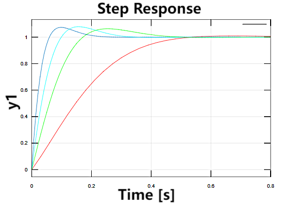
Figure 12. The step responses for different \( {K_{p}} \) values

On the step response graph, as shown in Figure 12, it can be observed that as \( {K_{p}} \) increases, the system's response speed also increases, accompanied by varying degrees of overshoot.

4. Discussion

A significant limitation lies in the simulation-based nature of these experiments (e.g., Tinkercad and Octave), as opposed to actual deployment on embedded systems or real-time control platforms. This disparity might introduce certain biases, potentially leading to variations between simulation results and real-world scenarios. The experiments utilized simplified P and PI control algorithms for the sake of simulation and comparative analysis. Nevertheless, practical applications often involve more intricate control algorithms. To address these limitations, future research could emphasize the validation of my findings on real embedded systems, consideration of more complex control algorithms, and a broader range of real-world application scenarios.

5. Conclusion

In the simulation of proportional feedback control, the analysis of the step response graphs reveals that as the value of \( {K_{p}} \) increases, the system's response time decreases, accompanied by a growing number of overshoots. An unstable system results in sustained oscillations rather than a gradual convergence to a steady state. A decrease in damping ratio typically indicates an enhanced tendency for system oscillation, potentially leading to more pronounced oscillations, larger oscillation amplitudes, and shorter settling times. The oscillation frequency is determined by the imaginary part. This could negatively affect system performance and stability. Hence, careful consideration of damping ratio selection is necessary in control system design to balance fast response and stability according to specific application requirements and performance goals. In the simulation of proportional-integral (PI) control, poles and zeros for different \( {K_{p}} \) values are all located in the left half of the complex plane with negative real parts, indicating system stability. On the PZmap, the length of the ellipse along the imaginary axis is greater than along the real axis, and with increasing \( {K_{p}} \) values, the points on the ellipse move further away from the real axis. However, after a certain \( {K_{p}} \) value, these points start to move closer to the real axis, reflecting changes in the frequency response characteristics of the PI control system. Compared to the step response of proportional feedback control, the degree of system oscillation significantly decreases. This indicates that introducing integral control into proportional feedback control helps make the system more stable, allowing for a relatively fast response while enhancing stability.

References

[1]. K.J. Åström, T. Hägglund, The future of PID control, Control Engineering Practice, Volume 9, Issue 11, 2001, Pages 1163-1175, ISSN 0967-0661.
[2]. Z.Shafiei, A.T. Shenton, Tuning of PID-type controllers for stable and unstable systems with time delay, Automatica, Volume 30, Issue 10, 1994, Pages 1609-1615, ISSN 0005-1098.
[3]. Ziegler, J. G. and N. B. Nichols (1942). Optimum setting for automatic controllers. Trans. ASME, 64, 759-768.
[4]. Anon, A. (1999). Special edition on PID tuning methods. Computing & Control Engineering Journal, 10(2).
[5]. Ho, M. T., Datta, A., & Bhattacharyya, S. P. (1996). A new approach to feedback stabilization. In Proceedings of the 35th IEEE conference on decision and control, IEEE, vol. 4 (pp. 4643–4648).
[6]. Munro, N., Söylemez, M. T., & Baki, H. (1999). Computation of D-stabilizing low-order compensators. IEEE Trans. on Automatic Control, Submitted for publication.
[7]. Söylemez, M. T., Munro, N., Baki, H. (1999). Fast calculation of stabilizing PID controllers. Automatica, submitted for publication.
[8]. Clark, D. W. (1986). Automatic tuning of PID regulators, in Expert Systems and Optimisation in Process Control, pp. 85-104. Technical Press.
[9]. Panagopoulos, H. (2000). PID control design, extension, application. Ph.D. thesis, Department of Automatic Control, Lund Institute of Technology, Lund, Sweden.
[10]. Wallen, A. (2000). Tools for autonomous process control. Ph.D. thesis, Department of Automatic Control, Lund Institute of Technology, Lund, Sweden.
[11]. Hao Yuan, et al., 2021. A fuzzy logic PI control with feedforward compensation for hydrogen pressure in vehicular fuel cell system, International Journal of Hydrogen Energy, Volume 46, Issue 7, Pages 5714-5728, ISSN 0360-3199.
[12]. Y. Li et al., 2021 "Electrochemical Model-Based Fast Charging: Physical Constraint-Triggered PI Control," in IEEE Transactions on Energy Conversion, vol. 36, no. 4, pp. 3208-3220.
[13]. Z. Li and S. Li, "Saturated PI Control for Nonlinear System With Provable Convergence: An Optimization Perspective," in IEEE Transactions on Circuits and Systems II: Express Briefs, vol. 68, no. 2, pp. 742-746, Feb. 2021, doi: 10.1109/TCSII.2020.3007879.
Cite this article
Long,J. (2023). Performance analysis of proportional feedback control and integral control in DC motors and speed control. Theoretical and Natural Science,26,81-88.
Data availability
The datasets used and/or analyzed during the current study will be available from the authors upon reasonable request.
Disclaimer/Publisher's Note
The statements, opinions and data contained in all publications are solely those of the individual author(s) and contributor(s) and not of EWA Publishing and/or the editor(s). EWA Publishing and/or the editor(s) disclaim responsibility for any injury to people or property resulting from any ideas, methods, instructions or products referred to in the content.
About volume
Volume title: Proceedings of the 3rd International Conference on Computing Innovation and Applied Physics
© 2024 by the author(s). Licensee EWA Publishing, Oxford, UK. This article is an open access article distributed under the terms and
conditions of the Creative Commons Attribution (CC BY) license. Authors who
publish this series agree to the following terms:
1. Authors retain copyright and grant the series right of first publication with the work simultaneously licensed under a Creative Commons
Attribution License that allows others to share the work with an acknowledgment of the work's authorship and initial publication in this
series.
2. Authors are able to enter into separate, additional contractual arrangements for the non-exclusive distribution of the series's published
version of the work (e.g., post it to an institutional repository or publish it in a book), with an acknowledgment of its initial
publication in this series.
3. Authors are permitted and encouraged to post their work online (e.g., in institutional repositories or on their website) prior to and
during the submission process, as it can lead to productive exchanges, as well as earlier and greater citation of published work (See
Open access policy for details).