1. Introduction

Forecasting housing price index is a classic problem in real estate and investment fields which can assist enterprises in adjusting investment strategy, help house buyers make sensible decisions and aid the government in promulgating policy. This paper will forecast the house price index for California with some models based on R studio.

When considering the impact of economic factors on housing price index, in 1994, John M. as well as Carmelo applied the method of repeat sales and the assessed value method and then concluded that the combination of two variables (like inflation and unemployment) can be beneficial to forecasting house price changes with the AV model [1]. David and Jack found that it is difficult to identify one particular variable or a very small number of variables that are able to forecast the housing price in 2007 [2]. In similar directions, in 2016, Wei and Cao concluded that no single factor has absolute superiority over others in forecasting the housing price since the best predictors change over time [3]. Bork and Moller applied the Dynamic Model Averaging and Dynamic Model Selection and found that the best predictors vary during different time periods [4]. These previous researches suggest that we should consider the interaction between multiple variables while researching and the result of forecast the housing price index will help the government make policy change, which is supposed by Chen, Cheng and Mao that will have influence on the housing price in the future [5].

When it comes to the models that have been used in previous studies, in 2010, Gu et al. presented a hybrid of genetic algorithm and support vector machines (G-SVM) approach to predict the housing price in China [6]. Then Gupta et al. combined the Ensemble Empirical Mode Decomposition model with the Support Vector Regression methodology to forecast the housing price of the US in 2014 and found that the accuracy of this EEMD-EN-SVR model is higher than that of the Random Walk model [7]. After that, the integration of Entropy and ANN presented by K. C. LAM, et al. forecasted the housing price in Hong Kong [8]. While the ANN model performed better when the size of sample is relatively small and the number of variables is suitable, so the optimal number of variables should be found before applying this model. By the way, the similar model (ANN) was proved to be accurate in forecasting in 2016 by Lim et al. [9]. In 2018, the fusion of Step-wise and SVM model was supposed to be a competitive approach and was applied to forecast the housing price in Melbourne by Phan [10]. Although the accuracy of these models is beyond doubt, they are all complicated and some of them require users to find the optimal sample number or other things that needed in the model before using, which adds difficulty in applying them.

This paper will use the simple forecast models in time series to predict the housing price index in California (a more detailed region), take multiple variables into account and see their effect, then combine the results from the two parts, give a general forecast value for the all state by checking the residuals of those simple models and select the most accurate one and then improve the accuracy of the results by increasing or decreasing certain values based on different regional situations (for instance, the region that has high average income per capita may receive some increasing in the predict value). This paper aims to use models that are easy to be explained to provide prediction for the index of housing price in California and optimize the forecast by considering the effect of multiple variables.

2. Methods

2.1. Data sources

The data of house price index in California for this paper is collected from the Federal Reserve Economic Data Website, which is a quarterly data and collect the observation from 1975.1.1 to 2023.4.1. Other data that may be related to house price index such as unemployment rate, income and population are also downloaded from this website.

2.2. Indicator selection and description

The FHFA House Price Index is an integrated set of the indexes of housing price collected from the public that gauge variation in single-family home values based on data that trace back to the mid-1970s from all fifty states and more than four hundred American cities. In this paper, we forecast this data to predict the future trend of house price in California.

In order to optimize our forecast, this paper choose some data that may be related to house price index and see if there is some relationship between them (Table 1).

Table 1. Variable description.

2.3. Research protocol

This paper uses four models for forecasting, including the mean model, the naïve model, the linear model, the drift model and the ARIMA model, and then test their accuracy for prediction in order to choose the most suitable one for forecasting the house price index in California. This paper then uses the multiple linear regression (MLR) to see if there is some relationship between the variables we assume and the predicted data.

2.4. Model principle

2.4.1. The mean model. Here, the predictions of all values in the future are equivalent to the average value of the previous data. If we denote the previous data by \( {y_{1}},{…,y_{T}} \) then we use \( { y_{T+h|T}} \) \( = \) \( ({y_{1}}+…+{y_{T}})÷T \) to express our predictions. The notation \( { y_{T+h|T}} \) is a short-hand for the assessment of \( { y_{T+h}} \) stem from the data \( {y_{1}},{…,y_{T}} \) .

2.4.2. The naïve model. In naive model, all predictions are simply considered to be equal to the value of the last observation, which can be expressed as \( {y_{T+h|T}} \) \( = \) \( {y_{T}} \) . This method usually works very well in some time series in economic and financial fields.

2.4.3. The drift model. Drift is considered as the value of variation over time. By considering the drift in the previous as the mean change in the whole data, the prediction for time  \( T+h \) is given by \( {y_{T+h|T}}={y_{T}}+\frac{h}{T-1}\sum _{t=2}^{T}({y_{t}}-{y_{t-1}})={y_{T}}+h(\frac{{y_{T}}-{y_{1}}}{T-1}) \) . The method is just like connecting a line between the first and last data points and extending the line along the timeline.

2.4.4. The ARIMA model. The ARIMA model (no seasonal) is the combination of autoregressive models and moving average models. Full equation of this model can be written as \( y_{t}^{,}=c+{∅_{1}}y_{t-1}^{,}+…+{∅_{p}}y_{t-p}^{,}+{θ_{1}}{ε_{t-1}}+…+{θ_{q}}{ε_{t-q}}+{ε_{t}} \) , where  \( {y_{t}} \) is the differenced series. Lagged values of  \( {y_{t}} \) and lagged errors are both included in the values of the forecasts. We call this an ARIMA \( (p,d,q) \) model.

2.4.5. The linear model. This model indicates a linear relationship between y and x, where y is the predicted variable and x is the predictor variable: \( {y_{t}}={β_{0}}+{β_{1}}{x_{t}}+{ε_{t}} \) The first coefficient  \( {β_{0}} \) represents the intercept of this line, and the gradient of this line is denoted by the second coefficient \( {β_{1}} \) . The intercept  \( {β_{0}} \)  shows what y equals when x is zero. The slope  \( {β_{1}} \)  shows the mean variation of y for each unit increase in x.

3. Results and discussion

3.1. Mean model

This paper firstly tests the mean model:

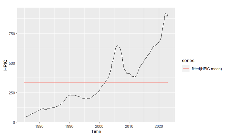
Figure 1. Fitted line of mean model

Table 2. Results of Ljung-Box test for mean model

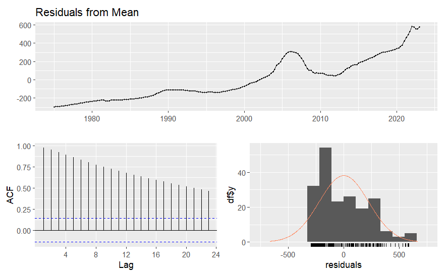
Figure 2. Residuals of mean model

From figure 1, we can see that the fitted line of the mean model is not close to the real data trend. From table 2, the Q value is very big from the Ljung-Box test. From figure 2, the average value of the residuals isn’t near 0, the lags have a strong trend in the ACF graph and the distribution of residuals isn’t close to the normal distribution, so the mean model isn’t a good model for forecasting this data.

3.2. Naïve model

This paper then tests the naïve model:

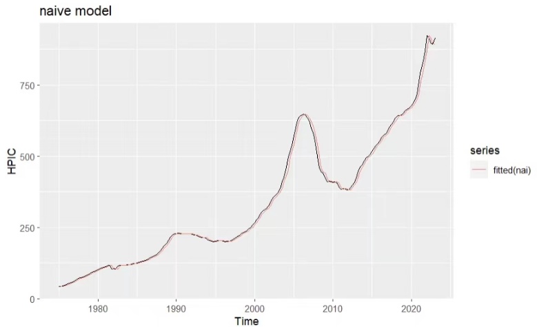
Figure 3. Fitted line of naïve model

Table 3. Results of Ljung-Box test for naïve model

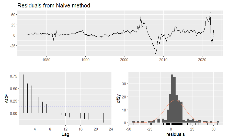
Figure 4. Residuals of naïve model

From figure 3, the fitted line of the naïve model is very close to the real data line. From table 3, the Q value is not very small. From figure 4, the average value of the residuals isn’t near 0, some of the lags exceed those blue lines interval in the ACF graph and the distribution of residuals is not very close to the normal distribution, so the naive model isn’t a suitable model for forecasting this data.

3.3. Drift model

Drift model is tested by using the data of house price index in California:

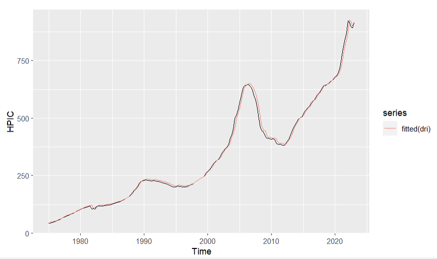
Figure 5. Fitted line of drift model

Table 4. Results of Ljung-Box test for drift model

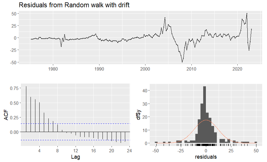
Figure 6. Residuals of drift model

From figure 5, the fitted line of drift model is close to the real data line. From table 4, the Q value of drift model is not very small. From figure 6, the average value of the residuals is close to 0, but some of the lags exceed the blue line interval in the ACF graph and the distribution of residuals isn’t very close to the normal distribution, so the drift model isn’t a suitable model for forecasting this data.

3.4. ARIMA model

ARIMA model is tested by using the data of house price index in California:

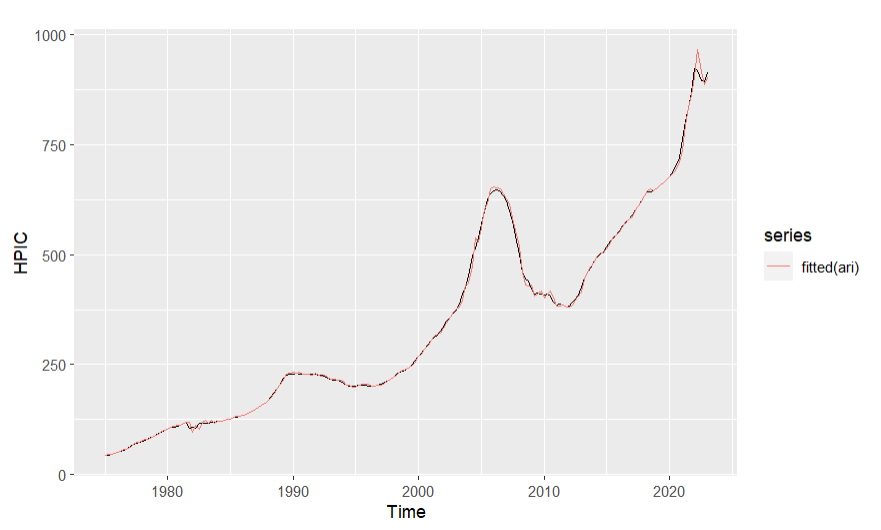
Figure 7. Fitted line of ARIMA model

Table 5. Results of Arima model

Table 6. Results of Ljung-Box test for ARIMA model

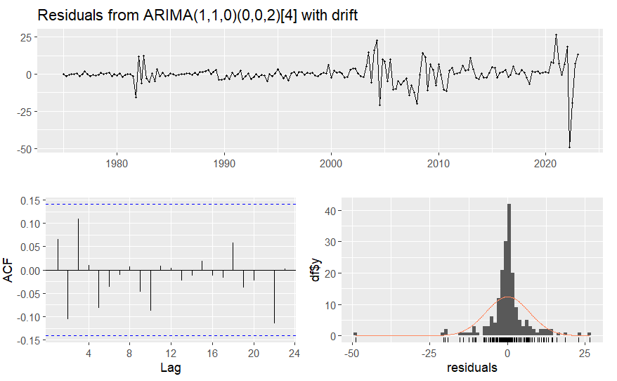
Figure 8. Residuals of ARIMA model

From table 5 and 6, the auto-ARIMA suggests us to use \( (1,1,0)(0,0,2) \) ARIMA model. From figure 7, the fitted line of ARIMA model is pretty close to the real data line. From table 5, the Q value is pretty small from the Ljung-Box. From figure 8, the average value of the residuals is close to 0, no lag exceed the blue line interval in the ACF graph, so the ARIMA \( (1,1,0)(0,0,2) \) model may be a good model for forecasting this data.

3.5. Linear model

Linear model is then tested in this paper:

Table 7. Results of linear regression model

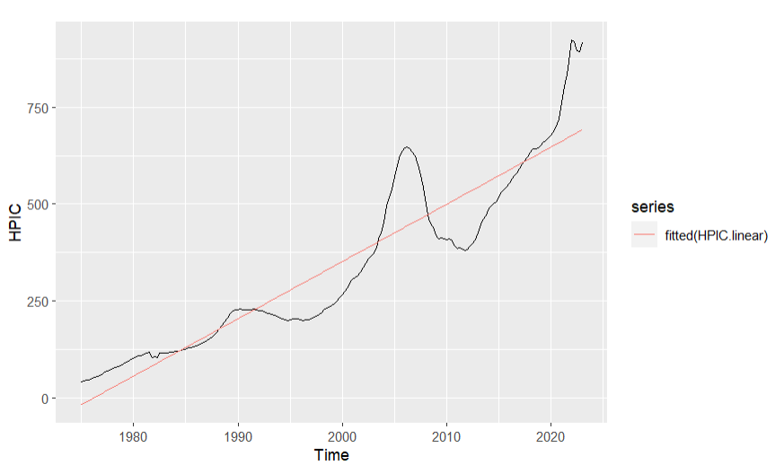
Figure 9. Fitted line of linear model

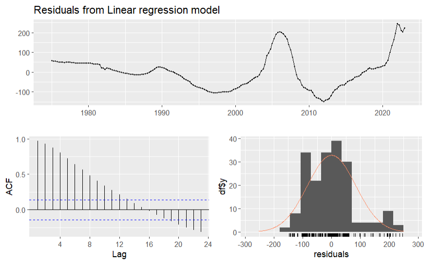
Figure 10. Residuals of linear model

From table 7, the equation between y and x is y=3.6876x-20.2655, the p value of the estimate of trend is between 0 and 0.001, which provide significant evidence for this model. From figure 9, the fitted line of the linear model is not close to the real data line. From figure 10, the average value of the residuals isn’t very close to 0, many of the lags exceed the blue line interval in the ACF graph and the distribution of residuals is not close to the normal distribution, so the linear regression model isn’t the suitable model for forecasting this data.

3.6. Forecast house price index

This paper has found that the ARIMA model is the most suitable model in the five simple models, so it is used for our final forecast:

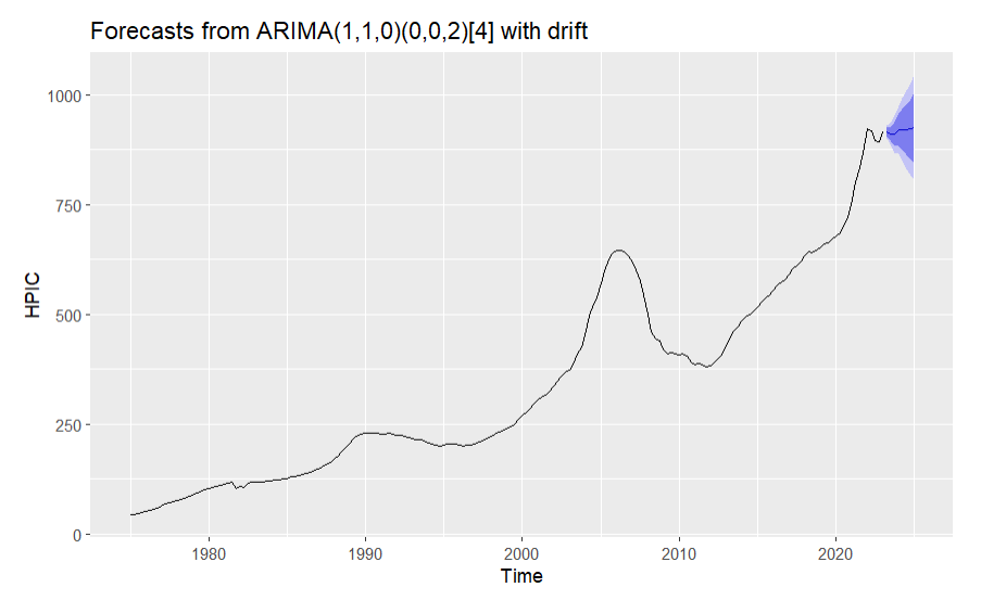
Figure 11. Forecasts from ARIMA model

From the forecasts in figure 11, the house price index in California in the next few years will be in the range from 850 to 1000.

3.7. Multiple linear regression

In this paper, we then use the multiple linear regression model in order to see if there is relationship between house price index in California, income per captia in California, unemployment rate in California and the population in California.

From the multiple linear regression results, the p value of population is pretty big, which is close to 1, while the p value of income and unemployment rate is pretty small (between 0 and 0.001), which provide significant evidence for the relationship between house price index and these two elements.

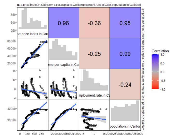
Figure 12. Correlation analysis chart

In order to see the complex relationship between these elements, this paper draw the correlation analysis chart by R studio. From figure 12, we can see that income and population have a strong relationship (because the r value between them is 0.99, which is very close to 1). House price index and income, house price and population also have strong relationship, with r value of 0.96 and 0.95 respectively. But the r value between house price index and unemployment rate is not very big (-0.36), which indicates that there is only weak correlation between these two elements, so unemployment rate in California may not be a good predict variable for the house price index in California.

4. Conclusion

By checking the residual of the models used in this paper, this paper found that the ARIMA model done the most accurate job in forecasting the house price index in California. By doing multiple linear regression with the house price index and three possible factors related to it, as well as drawing the correlation analysis chart between the four elements, this paper found that the income per captia in California not only shows high significance but also has strong correlation with the house price index in California, so it can be a useful predictor for house price index. Although the unemployment rate shows high significance in linear regression model, its correlation with house price index in not very strong, so it may not be a good predictor and the high significance may attribute to the large data volume. And the population also has strong correlation, but it doesn’t have high significance, which may because there is a non-linear relationship between these two elements. In conclusion, this paper will use the ARIMA model to predict the house price index in California in the next few years and consider income per captia in California as a predict factor to optimize the results.

By combining the forecast model and the multiple linear regression, in the region that has higher income per captia as well as higher population, the house price index will be higher, may be around 950, and in the region with lower income per captia as well as lower population, the house price index will be lower, may be around 850. There may be other factors that have effects on the house price index as well as more detailed data to do research with. In the future, if more time and data are provided, more variables are considered, the forecast may become more accurate and more useful.

References

[1]. John M 1994 The Influence of Economic Variables on Local House Price Dynamics. Journal of Urban Economics, 36, 161-183.
[2]. David E and Jack K 2007 Forecasting Real Housing Price Growth in the Eighth District States. Federal Reserve Bank of St. Louis Regional Economic Development, 3(2), 33-42.
[3]. Wei Y and Cao Y 2017 Forecasting house prices using dynamic model averaging approach: Evidence from China. Economic Modelling, 61, 147–155.
[4]. Lasse B and Stig V 2015 Forecasting house prices in the 50 states using Dynamic Model Averaging and Dynamic Model Selection. International Journal of Forecasting, 31, 63–78.
[5]. Chen N K, et al. 2014 Identifying and forecasting house prices: a macroeconomic perspective. Quantitative Finance, 2105-2120.
[6]. Gu, et al. 2011 Housing price forecasting based on genetic algorithm and support vector machine. Expert Systems with Applications, 38, 3383–3386.
[7]. Gupta, et al. 2015 Forecasting the U.S. real house price index. Economic Modelling, 45, 259–267.
[8]. Lam K C, et al. 2008 An Artificial Neural Network and Entropy Model for Residential Property Price Forecasting in Hong Kong. Journal of Property Research, 25(4), 321–342.
[9]. Lim, et al. 2016 Housing Price Prediction Using Neural Networks. 2016 12th International Conference on Natural Computation, Fuzzy Systems and Knowledge Discovery (ICNC-FSKD).
[10]. Danh P 2018 Housing Price Prediction using Machine Learning Algorithms: The Case of Melbourne City, Australia. 2018 International Conference on Machine Learning and Data Engineering (iCMLDE).
Cite this article
Zhang,Q. (2023). Forecast the house price index for California using different forecasting methods. Theoretical and Natural Science,26,95-104.
Data availability
The datasets used and/or analyzed during the current study will be available from the authors upon reasonable request.
Disclaimer/Publisher's Note
The statements, opinions and data contained in all publications are solely those of the individual author(s) and contributor(s) and not of EWA Publishing and/or the editor(s). EWA Publishing and/or the editor(s) disclaim responsibility for any injury to people or property resulting from any ideas, methods, instructions or products referred to in the content.
About volume
Volume title: Proceedings of the 3rd International Conference on Computing Innovation and Applied Physics
© 2024 by the author(s). Licensee EWA Publishing, Oxford, UK. This article is an open access article distributed under the terms and
conditions of the Creative Commons Attribution (CC BY) license. Authors who
publish this series agree to the following terms:
1. Authors retain copyright and grant the series right of first publication with the work simultaneously licensed under a Creative Commons
Attribution License that allows others to share the work with an acknowledgment of the work's authorship and initial publication in this
series.
2. Authors are able to enter into separate, additional contractual arrangements for the non-exclusive distribution of the series's published
version of the work (e.g., post it to an institutional repository or publish it in a book), with an acknowledgment of its initial
publication in this series.
3. Authors are permitted and encouraged to post their work online (e.g., in institutional repositories or on their website) prior to and
during the submission process, as it can lead to productive exchanges, as well as earlier and greater citation of published work (See
Open access policy for details).