1. Introduction

The harmonic oscillator is a system that is ubiquitous in physics. It approximately describes the systems from the classical pendulum to the molecular vibration. The study of the harmonic oscillator is important because any system in a stable equilibrium state can be approximated as a harmonic oscillator around that equilibrium point. Since classical harmonic oscillator treat the energy level as continuous, it does not work in quantum mechanics. Therefore, quantum harmonic oscillator (QHO) is a crucial step to understand the quantum world.

Classic quantum mechanics is not unified with the special relativity since Schrödinger Equation is not consist under Lorentz transformation. Klein-Gordon Field (KGF) equation is one of the first approach to unify quantum mechanics and special relativity. It is introduced to describe the relativistic spinless particle [1]. Nowadays, researchers focus on the quantization of generalized KGF for further study in curved space-time [2,3], and also focus on the solution of KGF with different boundary condition [4,5]. The numerical solution of KGF is also given by several researchers using different method [6,7]. A significant issue that occurs when scientists want to describe the particle more precise with the Klein-Gordon Equation is that it lacks positive definiteness [8]. Negative probability density could be derived from the KGF [9]. Therefore, further study of the KGF is needed. Quantum Field Theory (QFT) presents a novel framework for investigating the quantum realm. Quantized KGF, which is one of the main parts of QFT, resolve the problems given by KGF.

This paper will first discuss the quantization of classical harmonic oscillator and then briefly introduce the QFT. Finally, the author will introduce KGF and then discuss the quantization of KGF and present how the quantized harmonic oscillator makes a crucial part in the Quantized KGF.

2. Classical Harmonic Oscillator

Classical harmonic oscillator (CHO) describes the motion of a particle near the equilibrium point only lying in a potential field. The potential field can thus be approximate as a quadratic function of the position of the particle \( V(x)≈\frac{1}{2}m{ω^{2}}{x^{2}} \) . Since all external force is considered in the potential field, the Lagrangian of the system can be represent as kinetic energy minus potential energy

\( L=T-V=\frac{1}{2}m\dot{{x^{2}}}-\frac{1}{2}m{ω^{2}}{x^{2}}.\ \ \ (1) \)

Lagrangian of the system is a functional of the generalized coordinate \( x \) and their corresponding generalized velocity \( \dot{x} \) . According to the least action principle, the motion of the harmonic oscillator system is the one that minimize the action of the system, which is the integral of the Lagrangian over time: \( S=\int Lⅆt \) . This process gives the Euler-Lagrange equation \( \frac{d}{dt}(\frac{∂L}{∂\dot{x}})-\frac{∂L}{∂x}=0 \) , which minimize the action. Then the motion equation of the system is

\( \ddot{x}+{ω^{2}}x=0.\ \ \ (2) \)

The solution of Eq. (2) is

\( x(t)=Acos{(ωt+ϕ).}\ \ \ (3) \)

The value of \( A \) and \( ϕ \) are determined by the initial condition of the system, and the value of \( ω \) is determined by system itself. The motion of the system is an oscillation with frequency \( ω \) .

Since all force are derived from potential, Hamiltonian of the system is equivalent to the total energy of the system.

\( H=\frac{{p^{2}}}{2m}+\frac{1}{2}m{ω^{2}}{x^{2}}\ \ \ (4) \)

where \( p = mv \) is the momentum of the particle. Thus, the motion equation can also be derived from the Hamiltonian

\( \dot{x}={H_{p}}=\frac{p}{m},     \dot{p}=-{H_{x}}=-m{ω^{2}}x.\ \ \ (5) \)

3. Quantization of Harmonic Oscillator

CHO is a good approximation of motion near the equilibrium point. But in the situation that the quantum effect is significant, for example, the lattice vibration at low energies and velocities, CHO is not good. The wave-particle duality of the matter in system makes the position and momentum of it uncertain. Therefore, the matter in harmonic system can no longer be treated as particles with certain positions and momentums, it is more accurate to describe as waves. Quantum justification is then needed.

In quantum mechanics, the position and momentum are promoted to operators, which is a functional of the system states. It is found that

\( x→\hat{x}=xp→\hat{p}=-iℏ\frac{∂}{∂x}.\ \ \ (6) \)

The Hamiltonian operator of harmonic oscillator system is then

\( \hat{H}=\frac{{\hat{p}^{2}}}{2m}+\frac{1}{2}m{ω^{2}}{\hat{x}^{2}}.\ \ \ (7) \)

Apply this operator directly to a state which has stable energy state will not change the state. The Schrödinger equation then gives the time evolution of the system state

\( iℏ{ψ_{t}}=(\frac{{\hat{p}^{2}}}{2m}+\frac{1}{2}m{ω^{2}}{\hat{x}^{2}})ψ.\ \ \ (8) \)

Using ladder operator method, one can solve the Schrödinger equation easily. The ladder operator is defined as \( \hat{a}=\sqrt[]{\frac{mω}{2ℏ}}(\hat{x}+\frac{i}{mω}\hat{p}) \) . The summation, subtraction and multiplication of the ladder operator with its conjugate give the separation of position, momentum and Hamiltonian operator

\( \hat{x}=\sqrt[]{\frac{ℏ}{2mω}}(\hat{a}+{\hat{a}^{T}})       \hat{p}=-i\sqrt[]{\frac{mωℏ}{2}}(\hat{a}-{\hat{a}^{T}})        \hat{H}=ℏω(\hat{{a^{T}}\hat{a}}+\frac{1}{2})\ \ \ (9) \)

The commutation relations of those operators are shown in table 1.

Table 1. Commutation relation of operators.

4. Quantum Field Theory

When scientists walk into the region of high energy physics and high-speed physics, a theory that combine both relativity and quantum physics is needed. QFT, which grew out in the late 1920s, is the theory that unify quantum mechanics and special relativity [10]. In contract with other physical theories, there are no canonical definition for QFT. One of the best ways to understand the QFT is comparing it with other physical theories. In aspect of degree of freedom, QFT is an extension of quantum mechanics. QFT describes the system with infinite degree of freedom. In aspect of space-time, QFT is a theory that unify quantum mechanics with special relativity. Figure 1 shows the relation between classical mechanics, quantum mechanics, relativistic field theory and quantum field theory.

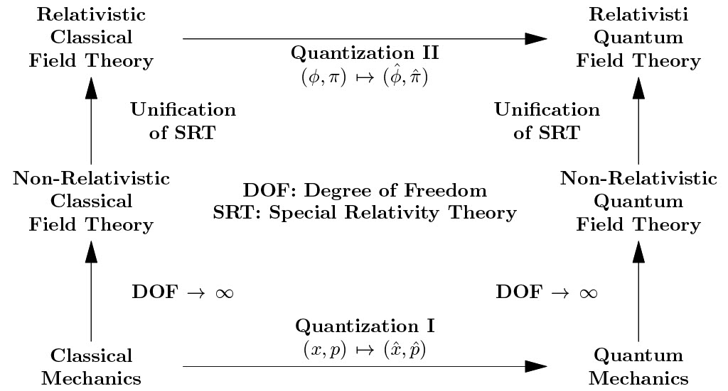
Figure 1. Relations between six major theories in modern physics.

5. Klein-Gordon Field

5.1. First Quantization of KGF

The KGF gives an approach to unify quantum mechanics and special relativity. It is obtained by apply energy-momentum relation \( {E^{2}}={p^{2}}{c^{2}}+{m^{2}}{c^{4}} \) to the Schrödinger equation. Promoting it to operator which analogous with quantization of harmonic oscillator and pluging into Schrödinger’s equation, it is found that

\( {\hat{E}^{2}}=-{ℏ^{2}}{c^{2}}{∇^{2}}+{m^{2}}{c^{4}}\ \ \ (10) \)

\( {(iℏ{∂_{t}})^{2}}ψ={\hat{E}^{2}}ψ=(-{ℏ^{2}}{c^{2}}{∇^{2}}+{m^{2}}{c^{4}})\ \ \ (11) \)

To follow the convention, changing equation into the natural unit, where \( ℏ= c = 1 \) , the field equation then becomes

\( (∂_{t}^{2}-{∇^{2}}+{m^{2}})ϕ=0.\ \ \ (12) \)

The \( ϕ \) here is a scalar field over space-time. i.e., it can be written as \( ϕ(t,x) \) . This is so called KGF Equation. It can represent the probability density to find the particle at point \( (t,x) \) in space-time. i.e., \( ⅆP={|ϕ(t,x)|^{2}}{ⅆ^{3}}xⅆt \) by the postulate of quantum mechanics. The equation can be simplified after Fourier transformation.

The Fourier transform of the KGF equation is

\( ϕ(t,x)=\int \frac{{d^{3}}kdω}{{(2π)^{3/2}}}{e^{ik\cdot x}}{e^{-iωt}}\widetilde{ϕ}(ω,k)\ \ \ (13) \)

The result after apply Fourier transformation into Eq. (12) is then

\( (-{ω^{2}}-{∇^{2}}+{m^{2}})\widetilde{ϕ}(ω,k)=0.\ \ \ (14) \)

Since consider a vanish solution is useless, the first term in the equation must be zero. i.e., \( {ω^{2}}=-{∇^{2}}+{m^{2}}≔ω_{k}^{2} \) is a function of momentum. The previous equation then becomes

\( (∂_{t}^{2}+ω_{k}^{2})ϕ=0.\ \ \ (15) \)

It became a simple harmonic oscillator equation with frequency \( {ω_{k}} \) . Eq3. (13) and (15) give the first quantization of KGF. At this stage, the field describes the state of a quantized particle. But it is not a quantum field yet. The field itself is still continuous. Since \( ϕ \) only non-vanishing at \( ω_{k}^{2}=-{∇^{2}}+{m^{2}} \) , it is convenient to introduce a delta function

\( \widetilde{ϕ}({ω_{k}},k)=δ({ω^{2}}-ω_{k}^{2})a({ω_{k}},k).\ \ \ (16) \)

The delta function has the property \( δ({ω^{2}}-ω_{k}^{2})=(δ(ω-{ω_{k}})+δ(ω+{ω_{k}}))/(2{ω_{k}}) \) , which is directly get from the definition of the delta function. Plug it into the Fourier transformation of the field equation and use the fact that KGF is a real-valued field, one can show that

\( ϕ(t,x)=\int \frac{{d^{3}}k}{{(2π)^{3/2}}}\frac{1}{2{ω_{k}}}({e^{-i{ω_{k}}t+ik\cdot x}}a({ω_{k}},k)+{e^{i{ω_{k}}t-ik\cdot x}}{a^{T}}({ω_{k}},k)), \ \ \ (17) \)

where \( a({ω_{k}},k) \) and \( {a^{T}}({ω_{k}},k) \) are then named as annihilation and creation operator of the field.

The solution of KGF can be interpreted as a continuous limit of lattice model. Consider a grid with separation \( a \) , and there is oscillator located in each grid point. This oscillator can be interpreted as a mass coupled with its nearest neighbour with spring and the equilibrium of the mass is at the centre of the grid. \( {ϕ_{a}}(t,x) \) for \( x \) in grid point is then the displacement of the mass from the equilibrium points at time \( t \) , which is also the state of oscillator at \( x \) . The KGF has the same form as \( \underset{a→0}{lim}{{ϕ_{a}}(t,x)} \) .

5.2. Second Quantization of KGF

Problems occur in this quantization of KGF. There is a confliction between localization and the positive definite of the energy of the field [9]. The second quantization of KGF is then introduced to solve those problems. The result of this quantization is same as quantize the oscillator in the lattice model in continuous limit, i.e., \( a→0 \) . This paper quantizes the KGF in canonical way.

To begin with, the Lagrangian L of the KGF is given by coordinate integral of the Lagrangian density over space \( ,L=\int {d^{3}}xL \) , where lagrangian density \( L(x) \) in the field is the subtraction of kinetic energy and potential energy at position x. i.e.,

\( L=\frac{1}{2}({∂_{μ}}ϕ{∂^{μ}}ϕ-{m^{2}}{ϕ^{2}}).\ \ \ (18) \)

The conjugate momentum of the field is then the partial derivative of the Lagrangian density with respect to time derivative of the coordinate function \( ϕ \) is \( π=\frac{∂L}{∂\dot{ϕ}}=\dot{ϕ} \) . The coordinate wave function \( ϕ \) and the conjugate momentum \( π \) are then promoted to operators \( \hat{ϕ} \) and \( \hat{π} \) . \( \hat{ϕ}(t,x) \) and \( \hat{π}(t,x) \) then represent the coordinate and momentum observable of the quantum field at time \( t \) and position \( x \) respectively. While those operators are applied, the whole field will collapse into a state that the coordinate or momentum of the field is certain depending on which operator is applied. Thus, it is crucial to understand how the canonical operators \( \hat{ϕ} \) and \( \hat{π} \) impact the field and how the effect of any other interested operators differ from them, which can be derived from the commutation relation between those operators and canonical operator. Therefore, to understand how the second quantization of KGF describes the physical world, it is necessary to examine the commutation relations of the canonical operators first. From Eqs. (17) and (18), the commutation relations in Table 2 can be derived [9].

Table 2. Commutation Relations of Some Operators in KGF.

The energy eigenstate can be derived from Hamiltonian operator H. The Hamiltonian of a field is the special integral of the Hamiltonian density \( H=\int Hⅆ{x^{3}} \) , where the harmiltonian density could derived from the lagrangian density of the field, \( H=π\dot{ϕ}-L \) . This gives

\( H=\frac{1}{2}{π^{2}}+\frac{1}{2}{(∇ϕ)^{2}}+\frac{1}{2}{m^{2}}{ϕ^{2}}\ \ \ (19) \)

The integration of Hamiltonian density over the space gives a concise result when it is expressed by ladder operators

\( H=\frac{1}{2}\int {d^{3}}k{ω_{k}}(a(k){a^{T}}(k)+{a^{T}}(k)a(k))\ \ \ (20) \)

The commutation relation between Hamiltonian and ladder operators is thus obtained. Namely, they are \( [\hat{H},\hat{a}(k)]=-{ω_{k}}\hat{a} \) and \( [\hat{H},{\hat{a}^{T}}(k)]={ω_{k}}{\hat{a}^{T}} \) . These relations infer that applying \( \hat{a}(k) \) to the field will decrease the energy with \( {ω_{k}} \) for any activated state. By contrast, applying \( {\hat{a}^{T}}(k) \) will increase the energy with \( {ω_{k}} \) . Therefore, like the ladder operator in QHO, \( {\hat{a}^{T}}(k) \) excite the field with a particle that have momentum k and \( \hat{a}(k) \) annihilate the particle with momentum \( k \) .

6. Conclusion

An unsolvable conflict occurs after applying energy-momentum relation to the Schrödinger equation gives the KGF. To solve this conflict, this paper uses canonical quantization method. This method interprets the field as a grid that the gap of grid is infinitesimal. Each grid contains a mass that oscillate around its equilibrium. The value of field at each position is interpreted as the distance of the mass from its equilibrium. While the KGF is used to solve quantum problems, which is the purpose physicists introduce it, the oscillator in each position should be quantized. This interpretation of the KGF gives a similarity between quantized KGF and QHO. The coordinate operator \( \hat{ϕ}(t,x) \) is analogous to the position operator \( \hat{x} \) ; the conjugate momentum operator \( \hat{π}(t,x) \) is analogous to the momentum operator \( \hat{p} \) and the annihilation and creation operator \( a(k) \) and \( {a^{T}}(k) \) are analogous to the ladder operator \( \hat{a} \) and \( {\hat{a}^{T}} \) . The behavior of field operators is same as the classic quantum operator when constrict those operators to a certain position and momentum, and always commutate with each other in different position or momentum. This decoupling of the position supports the interpretation of the KGF.

References

[1]. Poveda LA, Grave de Peralta L, Pittman J, Poirier B. (2022). A Non-relativistic Approach to Relativistic Quantum Mechanics: The Case of the Harmonic Oscillator. Found Phys 52(1), 29.
[2]. Ahmed F. (2020). Klein-Gordon Oscillator in the Presence of External Fields in a Cosmic Space-Time with a Space-Like Dislocation and Aharonov-Bohm Effect. Adv High Energy Phys 2020, 1–10.
[3]. Harikumar E, Rajagopal V. (2019). Quantisation of Klein–Gordon field in κ space-time: deformed oscillators and Unruh effect. Eur Phys J C 79, 735.
[4]. Dappiaggi C, Ferreira HRC, Marta A. (2018). Ground states of a Klein-Gordon field with Robin boundary conditions in global anti–de Sitter spacetime. Phys Rev D 98, 025005.
[5]. George A. (2005). The massive Klein–Gordon field coupled to a harmonic oscillator at the boundary. J Phys Math Gen 38, 7399–7418.
[6]. Balogh A, Banda J, Yagdjian K. (2019). High-performance implementation of a Runge–Kutta finite-difference scheme for the Higgs boson equation in the de Sitter spacetime. Commun. Nonlinear Sci. Numer. Simul. 68, 15–30.
[7]. Wang H. (2019). Numerical simulation for solitary wave of Klein–Gordon–Zakharov equation based on the lattice Boltzmann model. Comput. Math. Appl. 78, 3941–3955.
[8]. Bao W, Dong X. (2012). Analysis and comparison of numerical methods for the Klein–Gordon equation in the nonrelativistic limit regime. Numer. Math. 120:189–229.
[9]. Strocchi F. (2013). Relativistic quantum mechanics. In: Strocchi F (ed) An Introduction to Non-Perturbative Foundations of Quantum Field Theory. Oxford University Press.
[10]. Weinberg S. (1977). The Search for Unity: Notes for a History of Quantum Field Theory. Daedalus 106, 17–35.
Cite this article
Wu,K. (2023). Embarking on the path to quantum field theory. Theoretical and Natural Science,26,221-226.
Data availability
The datasets used and/or analyzed during the current study will be available from the authors upon reasonable request.
Disclaimer/Publisher's Note
The statements, opinions and data contained in all publications are solely those of the individual author(s) and contributor(s) and not of EWA Publishing and/or the editor(s). EWA Publishing and/or the editor(s) disclaim responsibility for any injury to people or property resulting from any ideas, methods, instructions or products referred to in the content.
About volume
Volume title: Proceedings of the 3rd International Conference on Computing Innovation and Applied Physics
© 2024 by the author(s). Licensee EWA Publishing, Oxford, UK. This article is an open access article distributed under the terms and
conditions of the Creative Commons Attribution (CC BY) license. Authors who
publish this series agree to the following terms:
1. Authors retain copyright and grant the series right of first publication with the work simultaneously licensed under a Creative Commons
Attribution License that allows others to share the work with an acknowledgment of the work's authorship and initial publication in this
series.
2. Authors are able to enter into separate, additional contractual arrangements for the non-exclusive distribution of the series's published
version of the work (e.g., post it to an institutional repository or publish it in a book), with an acknowledgment of its initial
publication in this series.
3. Authors are permitted and encouraged to post their work online (e.g., in institutional repositories or on their website) prior to and
during the submission process, as it can lead to productive exchanges, as well as earlier and greater citation of published work (See
Open access policy for details).