1. Introduction

Population forecasting has consistently ranked among the most prominent subjects in social science research. Precise population forecast data carries substantial societal benefits. For governments, an accurate grasp of future population trends aids in crafting effective welfare policies, planning agricultural production, and managing water resource reserves. Likewise, businesses can make informed decisions by leveraging insights into population dynamics. By tailoring marketing strategies, companies can secure enhanced profits, thereby fostering both socio-economic progress and development.

When dealing with population, a variable influenced by multifaceted factors, the autoregressive model is the first methodology that comes to mind. Cesario et al. introduced its application in predicting the criminal population in a district of Chicago, USA [1]. This model effectively combines trend and seasonality components. By isolating these elements, the remaining error behaves as white noise. The resulting autoregressive model demonstrated commendable performance, yielding a forecast error of 16% over one year. Over two years, the margin of error expanded to 20%. Regrettably, the model does not incorporate factors affecting crime rates, rendering it heavily reliant on historical crime data. This oversimplification in structure is a notable limitation.

Apart from the autoregressive model, classical approaches for population forecasting encompass Simple Exponential Smoothing (SES), Holt Exponential Smoothing (HES), and ARIMA models. In their study, Chen et al. compared the predictions of the criminal population in various Chinese cities using these three methods [2]. Their findings indicated that the ARIMA model (explained further in this paper) exhibited a lower Root Mean Square Error (RMSE), underscoring its advantage over the other two models due to its more sophisticated architecture.

On a related note, dynamic models factor in additional linear components, representing a fusion of ARIMA and multiple linear regression models. Box et al. exemplified this approach in predicting electricity consumption among German consumers [3]. Compared with the averaging method employed by e-commerce, it was discerned that the optimal model incorporated the STL method for modelling trend and seasonal elements.

Dynamic regression models, elaborated by George et al., found a wide range of applications, especially those developed based on ARIMA models [4]. However, there is a lack of literature addressing population prediction problems in dynamic regression models. This paper aims to bridge this gap and open new avenues for population prediction models. The approach in this paper employs an enhanced dynamic model based on time series concepts to forecast the total U.S. population. This model combines historical population data with influencing factors to improve the accuracy of predicting future population changes. The author believes that dynamic models describe population trends more accurately than static models. External factors such as unemployment, personal disposable income, and the number of families with couples can considerably impact population size. Furthermore, the author believes that these factors may interact. This report will first describe the data sources and processing methods and then explain the model construction principles. Subsequently, the validity of the model fit will be demonstrated and evaluated. Finally, this report will present the conclusions of this report and suggest potential directions for future research.

2. Methodology

2.1. Data source

In this study, a total of 15 variables were examined, and the majority of the data in this report was sourced from websites belonging to various U.S. government agencies. Specifically, the data pertaining to the primary research objective, which is the growth of the U.S. population, was obtained from the United States Census Bureau. The remaining 14 explanatory factors were collected from a range of sources, including the Centers for Disease Control and Prevention, U.S. Census Bureau, U.S. Bureau of Labor Statistics, U.S. Bureau of Economic Analysis, Federal Bureau of Investigation, FRED Economic Data, U.S. Department of Homeland Security, and Macrotrends. Information for all 15 variables is contained in a single database, and the data in each database is numerical. For each variable, 38 years of data from 1984 to 2020 are used in this report. The data is divided into the training and test sets as shown in figure 1.

Figure 1. Data classification

Since all variables are based on data for the entire United States, we believe these data are reasonable, so we do not analyse outliers. We used the Last Observation Carried Backward (LOCB) method for the few missing values. This method is a common method for dealing with trended time series. It supplements the previous year's data with the year's data with missing values. Using this method does not introduce much error in the results for small numbers of missing values.

The U.S. population annually is in the millions. The data is sourced from the population estimate from the Census Bureau by the 1st of July every year. CPI: The consumer price index is defined as the change in prices paid by U.S. consumers, which measures the cost of living in the United States. GDP: Gross Domestic Income is the indicator of the nation's overall economic health. The number of family households with married couples in thousand. Number of legal immigrants every year. The average price for rice, white, long grain, uncooked (cost per Pound) in U.S. city average in Dollars. National Health Expenditure (amount in billions of dollars). Annual Real Median Household Income in the U.S. (in adjusted dollars). The Unemployment Rate (Percent) is measured in the number of unemployed people as a percentage of the labour force. Life expectancy at age 65. National query number of violent crime. Percentage of the population living on less than $5.50 a day at 2011 international prices. Percent distribution of vacant units of all kinds of housing units for each year.

2.2. Methodology introduction

First, this article will review the basic knowledge of dynamic models, and then introduce the methodology specific to the details of each part of Figure 2.

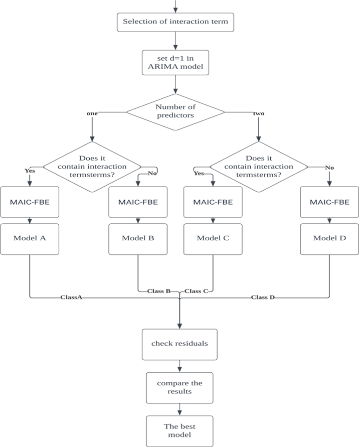
Figure 2. Methodology corresponding flow chart

Backshift notation is a convenient mathematical expression that will be widely cited in the following text [4].

\( B{y_{t}}={y_{t-1}}. \) (1)

\( {y_{t}} \prime ={y_{t}}-{y_{t-1}}={y_{t}}-B{y_{t}}=(1-B){y_{t}} \) (2)

\( {{(1-B)^{d}} y_{t}}={y_{t-d}} \) (3)

The dynamic regression model is synthesized based on the ARIMA model and the linear model. This model combines two models, namely Autoregression models and Moving average models. This model has a clear mathematical basis and can accurately capture the autocorrelation and average structure of time series. also. This model only requires a set of data of observed variables to make predictions, and the parameters can be flexibly adjusted, making it very easy to operate. Here is the formula for ARIMA:

\( {y_{t}} \prime =c+{ϕ_{1}}y{ \prime _{t-1}}+…+{ϕ_{p}}y{ \prime _{t-p}}+{θ_{1}}{ϵ_{t-1}}+…+{θ_{q}}{ϵ_{t-q}}+{ϵ_{t}} \) (4)

Where \( {y_{t}} \) is the series after one difference (in real-world questions, it may be higher than just once). According to [5], among ARIMA, ES, GRNN and ARIMA–GRNN hybrid models, the ARIMA model best predicts daily new COVID-19 cases in India.

However, for the complex forecasting goal of population change, it is one-sided to only focus on capturing the inherent autoregressive and average moving structures of time series. We need to introduce multiple regression models to provide some linear predictors for the prediction model. This is the formula of the multiple regression model:

\( {y_{t}}={β_{0}}+{β_{1}}{x_{1,t}}+{β_{2}}{x_{2,t}}+…+{β_{k}}{x_{k,t}}+{ϵ_{t}} \) (5)

Here, y is the response variable, and \( { x_{\lbrace 1,t\rbrace }},{x_{\lbrace 2,t\rbrace }},…,{x_{\lbrace k,t\rbrace }} \) are explanatory variables. For this model, Peter Martin in his book [6], takes the prediction of mental health as an example, the operation process of the multivariate linear model is explained in detail. Then, we can build the dynamic regression model with order (1,1,1):

\( {y_{t}}={β_{0}}+{β_{1}}{x_{1,t}}+…+{β_{k}}{x_{k,t}}+{η_{t}} \) (6)

\( (1-{ϕ_{1}}B)(1-B){η_{t}}=c+(1+{ϕ_{1}}B){ϵ_{t}} \) (7)

Literature has mentioned many examples of this model. In addition, we will introduce the concept of interaction term into the dynamic model [7]. For example, the two influencing factors of unemployment rate and poverty rate may influence and interact with each other. In addition, these two factors may affect population growth simultaneously. This is, the interaction term will be very convenient for predicting the term. After adding the interaction term \( {x_{1,t}}*{x_{2,t}} \) to improve the model, we get the model with order (1,1,1):

\( {y_{t}}={β_{0}}+{β_{1}}{x_{1,t}}*{x_{2,t}}+{β_{3}}{x_{3,t}}…+{β_{k}}{x_{k,t}}+{η_{t}} \) (8)

\( (1-{ϕ_{1}}B)(1-B){η_{t}}=c+(1+{ϕ_{1}}B){ϵ_{t}} \) (9)

At this point, the mathematical expression of the dynamic model of this study has been introduced. There are many assumptions used in this model. Linearity assumption: In dynamic models, a linear equation is assumed to describe the relationship between variables. Interaction assumption: The model assumes the presence of interactive effects between two or more variables, which change over time. This implies that the relationship between variables is not static but dynamic. Stability assumption: The model assumes that the relationship between variables remains relatively stable over the observation period, meaning that the effects of interactions do not fluctuate drastically with time. No omitted variable assumption: The model assumes no omitted variables influence the relationship between the variables. All factors affecting the relationship have been considered. Linear dynamics assumption: The model assumes that the dynamic effects of interactions can be modelled linearly. If the relationship between variables exhibits non-linear dynamic changes, more complex models or non-linear effects may need to be considered. White noise assumption: We assume the residuals are white noise, meaning they have a constant mean and variance and no autocorrelation.

Before introducing the four model frameworks proposed in this study, it is necessary to find the interaction terms. After observing the images of all predictors, there are two time series plots that are very similar in figure 3. They both reached the local lowest value in 1980 and the fluctuation frequencies are basically similar.

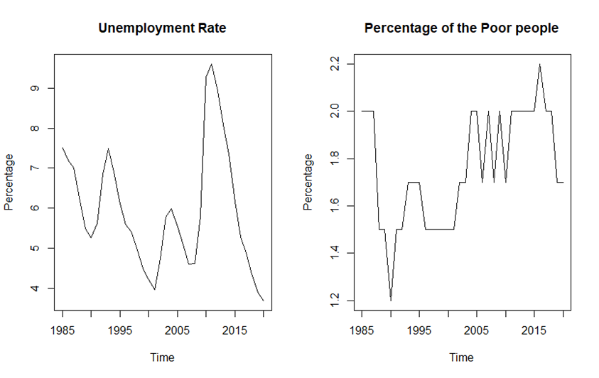
Figure 3. Time series plots of unemployment and poverty rates

In addition, these two variables influence each other in real life. An increase in the poverty rate will exacerbate the surge in unemployment. On the contrary, an increase in the unemployment rate will also directly affect the poverty rate. So, ultimately, this study chooses the Unemployment rate * Poverty rate as an interaction term

In order to select the best dynamic model, I designed four sets of models with different frameworks. They are a dynamic model with one predictor, a dynamic model with two predictors, a dynamic model with one predictor and a cross term, and a dynamic model with two predictors and a cross term. All four models used will use order d=1 to increase the stationarity of the data. Which model to choose as the optimal solution in each classification is the focus of the article. This study chooses to exhaust all the free combinations of variables exhaustively and then provides the Minimal AIC Method for Fact-Based Elimination (MAIC-FBE) to screen out the optimal model. This method will be presented after the introduction of AIC

The Akaike Information Criterion (AIC) is a model evaluation metric used for selecting the best model among several statistical models [8]. Here is the basic formula:

\( AIC=2k-2ln{(L)} \) (10)

k is the number of parameters (degrees of freedom) in the model and \( ln⁡(L) \) is the natural logarithm of the maximum likelihood estimate of the model. From the formula, we can find that AIC value will become large when k is high. This is to prevent overfitting by penalizing too many variables.

The MAIC-FBE method is to list all possible model situations and calculate the AIC value of each model. Then, take out the model with the lowest AIC value. If the parameters of this model meet practical significance, select this model as the optimal model of this framework. If the parameters of this model do not match the laws of real life, propose a secondary model and repeat the process. Finally, a model that conforms to the laws of real life and has the lowest AIC value will be screened out.

After selecting the optimal solutions for the four types of models and obtaining the final dynamic model through compare the test RMSE, this study also needs to analyse the residuals of the model. As the white noise assumption introduced above, if statisticians want to verify whether the residuals of the model have no autocorrelation, they may use the Ljung-Box test from [9]. Ljung-Box test is a statistical test used to examine whether there is autocorrelation in time series data. It is commonly employed to determine if there is significant autocorrelation at various lags. If the p-value of the Ljung-Box test is less than a predetermined significance level (typically set at 0.05), the null hypothesis is rejected indicating the presence of autocorrelation.

3. Result and discussion

The following four models are the optimal models of the abovementioned frameworks. They have the lowest AIC value among similar models.

Model A: Dynamic model with one predictor.

\( {y_{t}}=-0.0009*Crime+{η_{t}} \) (11)

\( (1-1.5224*B-0.6896*{B^{2}})(1-B){η_{t}}=2762.2688+{ϵ_{t}} \) (12)

Model B: Dynamic model with two predictors.

\( {y_{t}}=-0.0011*Crime-41.6998*Poverty+{η_{t}} \) (13)

\( (1-1.5368*B+0.7078*{B^{2}})(1-B){η_{t}}=2760.2364+{ϵ_{t}} \) (14)

Model C: Dynamic model with one predictor and an interaction term.

\( {y_{t}}=-18.7896*Unemp{l_{rate}}*Poverty-0.0015*Crime+{η_{t}} \) (15)

\( (1-0.8486*B)(1-B){η_{t}}=2654.0113+(1+0.9399*B){ϵ_{t}} \) (16)

Model D: Dynamic model with two predictors and an interaction term.

\( {y_{t}}=-9.0461*Unemp{l_{rate}}*Poverty-0.0012*Crime+10.0341*CPI+{η_{t}} \) (17)

\( (1-1.5299*B+0.7015*{B^{2}})(1-B){η_{t}}={2733.2221+ϵ_{t}} \) (18)

Table 1. Basic information about the four prediction models

The above table 1 is a summary of important information about the four models. It can be seen from table 1 that Model A has the lowest AIC value. However, the lowest AIC value does not mean it is the best model because AIC is penalised for multiple predictors. This leads to a high probability that the AIC value of Model C is higher than the AIC value of Model A and the AIC value of Model D is higher than the AIC value of Model B. Therefore, we introduced a new mathematical indicator, Root Mean Square Error (RMSE), to measure the fitting effect of the model. Suppose \( \hat{p} \) represents the numerical value of the fitted population, p represents the numerical value of the actual population. In this study:

\( RMSE(training)=\sqrt[]{\frac{1}{27}\sum _{i=1984}^{2010}{(\hat{{p_{i}}}-{p_{i}})^{2}}} \) (19)

\( RMSE(test)=\sqrt[]{\frac{1}{10}\sum _{i=2011}^{2022}{(\hat{{p_{i}}}-{p_{i}})^{2}}} \) (20)

In terms of the Root Mean Square Error (RMSE) on the training set, Model C outperformed the others with the lowest value of 118.0259. This suggests that Model C exhibits the most favourable fitting performance on the training data. Following closely, Model D achieved a value of 120.0354, indicating a fitting effect nearly on par with that of Model C. On the other hand, both Model A and Model B demonstrated comparatively weaker performance in this metric, registering scores of approximately 124 and 122, respectively.

Turning our attention to the RMSE on the test set, Model D showcased a substantial lead, surpassing the runner-up by more than double with a value of 590.2484 compared to 1167.364. Model A displayed a well-balanced performance and excelled in the test set given the predictor. However, in joint assessment, the superior model is Model D. This conclusion is rooted in the consideration that the RMSE of the test set holds the highest significance. This is because it directly gauges the model's predictive capability on external data, whereas the RMSE of the training set primarily reflects the model's fitting performance on the provided data.

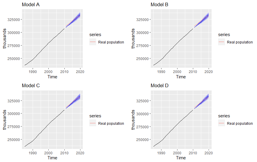
Figure 4. Comparison of prediction effect of four models

Through the prediction method mentioned in [10], we get Figure 4. For this figure, the light blue intervals of these four prediction maps are all 80% prediction intervals, and the dark blue intervals are 95%. We see that the four models all have large deviations in their prediction performance for data around 2012. For data around 2015, Model D’s predicted values are closer to the actual values. However, the other three models perform better for data around 2019. The prediction interval range of the four models increases with time, so the dynamic model is based on short- and medium-term prediction models. For the situation nine years after 2019, data scientists will not use dynamic models to predict. So, model D is the best model for dynamic models.

The optimal model formulas are (17) and (18). According to this expression, the future population will increase by an average of about 10,034 people for every unit of increase in CPI. For every crime reduction, the population increases by one. For every unit decrease in Unemployment rate *Poverty rate, the population is expected to increase by 9046 people. In order to analyse whether the model achieves white noise, we need to analyse the residuals. With the help of R language, we get the following Figure 5.

The first picture is a display of the residual time series. The second picture is the ACF chart used to measure autocorrelation between residuals. No value corresponding to Lag exceeds the critical interval, which means there is no autocorrelation between the data. In addition, if we perform the Ljung-Box test on residuals, we get a p-value of 0.1995, much larger than 0.05. We cannot reject the null hypothesis, so we double-verify that the residuals have no autocorrelation.

Model D was the final chosen dynamic model. However, from the perspective of the cumulative distribution of residuals, it does not follow the normal distribution and does not necessarily have the characteristic that the variance is constant. The prediction model D may not comply with white noise to a certain extent, affecting the final prediction results. In addition, according to Figure 4, the model's short-term fitting effect is not good, and further research is needed. However, Model D finally performed well in the test concentration period, and the prediction curve coincided with the natural population curve. Compared with [1] and [2], the model in this study is more accurate in mid-term prediction and enriches the model structure of dynamic models in population prediction. Future workers can study some methods to reduce the initial fitting error of the test set based on this model and try some nonlinear models.

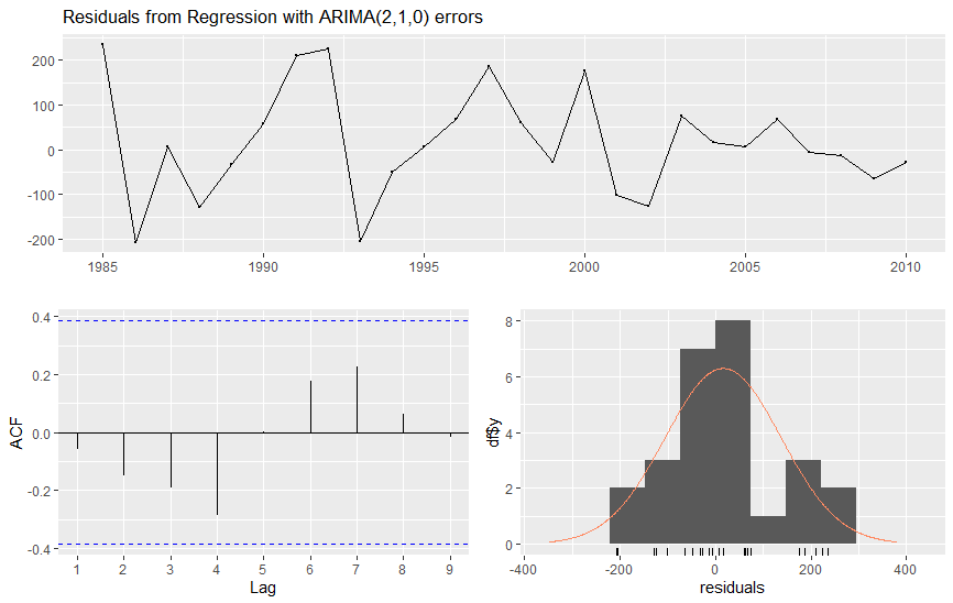
Figure 5. Residual analysis

4. Conclusion

Compared with most dynamic models that use seasonal analysis, the best model discussed in this report does not use this analysis method but uses direct analysis year by year. A total of 15 predicted shadows were tested to obtain the best dynamic model. Through classification, four structural models were repeatedly screened and iterated. After obtaining the four corresponding best models, Model D, with the lowest AIC value, was selected as the final dynamic model. The model shows that the unemployment, crime, CPI and poverty rates clearly correlate with the total population. It accurately predicts the total population in about five years, that is, around 2015. This article is of great importance for understanding dynamic models and methods for predicting populations. In addition, the best model, Model D, will help the government and social science departments further research and make more accurate predictions of the future U.S. population.

References

[1]. Cesario E, Catlett C and Talia D 2016 Forecasting crimes using autoregressive models. In 2016 IEEE 14th Intl Conf on Dependable, Autonomic and Secure Computing, 14th Intl Conf on Pervasive Intelligence and Computing, 795-802.
[2]. Chen P, Yuan H and Shu X 2008 Forecasting crime using the arima model. In 2008 fifth international conference on fuzzy systems and knowledge discovery, 5, 627-630.
[3]. Shaqiri F, Korn R and Truong H P 2023 Dynamic Regression Prediction Models for Customer Specific Electricity Consumption. Electricity, 4(2), 185-215.
[4]. Box G E, Jenkins G M, Reinsel G C and Ljung G M 2015 Time series analysis: forecasting and control. John Wiley & Sons.
[5]. Wang G, et al. 2021 Comparison of ARIMA, ES, GRNN and ARIMA–GRNN hybrid models to forecast the second wave of COVID-19 in India and the United States. Epidemiology & Infection, 149, 240.
[6]. Martin P 2022 Linear regression: An introduction to statistical models. Sage.
[7]. Shumway R H, Stoffer D S and Stoffer D S 2000 Time series analysis and its applications. New York: springer.
[8]. Akaike H 1974 A new look at the statistical model identification. IEEE transactions on automatic control, 19(6), 716-723.
[9]. Ljung G M and Box G E 1978 On a measure of lack of fit in time series models. Biometrika, 65(2), 297-303.
[10]. Hyndman R J and Athanasopoulos G 2018 Forecasting: principles and practice. OTexts.
Cite this article
Li,H. (2024). Application of dynamic models in forecasting the total population of the United States. Theoretical and Natural Science,30,50-58.
Data availability
The datasets used and/or analyzed during the current study will be available from the authors upon reasonable request.
Disclaimer/Publisher's Note
The statements, opinions and data contained in all publications are solely those of the individual author(s) and contributor(s) and not of EWA Publishing and/or the editor(s). EWA Publishing and/or the editor(s) disclaim responsibility for any injury to people or property resulting from any ideas, methods, instructions or products referred to in the content.
About volume
Volume title: Proceedings of the 3rd International Conference on Computing Innovation and Applied Physics
© 2024 by the author(s). Licensee EWA Publishing, Oxford, UK. This article is an open access article distributed under the terms and
conditions of the Creative Commons Attribution (CC BY) license. Authors who
publish this series agree to the following terms:
1. Authors retain copyright and grant the series right of first publication with the work simultaneously licensed under a Creative Commons
Attribution License that allows others to share the work with an acknowledgment of the work's authorship and initial publication in this
series.
2. Authors are able to enter into separate, additional contractual arrangements for the non-exclusive distribution of the series's published
version of the work (e.g., post it to an institutional repository or publish it in a book), with an acknowledgment of its initial
publication in this series.
3. Authors are permitted and encouraged to post their work online (e.g., in institutional repositories or on their website) prior to and
during the submission process, as it can lead to productive exchanges, as well as earlier and greater citation of published work (See
Open access policy for details).