1. Introduction

There has been a long line of work on the “coin weighing problem”. A stack of coins, each has weight either 0 or 1. There is a scale which tells you the total weight of an arbitrary subset of coins. A natural question: how to get the weight of each coin with as few weighing as possible? \( n \) weighing are definitely enough, but can we do better? The answer is positive. One can play with the problem a bit and find that 3 weighing is enough to figure out the weights of 4 coins. Due to the simplicity of the problem and its connection to group testing, this problem was almost resolved by mathematicians in 1960s. An important piece of work is by Lindström, in which they found a clever way to construct the queries and recovery the weights [1].

The query complexity of an algorithm with query access is defined as the number of queries the algorithm makes. Cantor and Mills designed the first \( O(n/log⁡n) \) query complexity algorithm for the coin weighing problem [2]. The algorithm is recursive and elegant. Lindström argued the coin weighing problem has query complexity \( Θ(n/log⁡n) \) [1]. The lower bound uses a combinatorial argument involving determinant of a family of matrices, although one can see the asymptotic lower bound \( Ω(n/log⁡n) \) nearly immediately by using some ideas from information theory: each query givens at most \( log⁡n \) bits of information, yet there are \( n \) bits of information hiding in \( x \) .

The study of coin weighing with arbitrary \( x \) was almost closed at this point. Since then, more refined groups of coins are conjured and studied. A notable one is the group of coins with total weights \( d \) . The coin family now has size \( (\begin{matrix}n \\ d \\ \end{matrix}) \) , while on the other hand each weighing gives at most \( log⁡d \) bits of information. The leads to a \( Ω\frac{dlog⁡(n/d)}{log⁡d} \) lower bound. The same upper bound is achieved by Bshouty with an adaptive, deterministic algorithm [3]. There are ongoing works on getting better non-adaptive algorithms, with the current best non-adaptive deterministic algorithm of query complexity \( O(dlog⁡n) \) , achieved by the BCH code, discovered separately by Raj Chandra Bose, Dwijendra Kumar RayChaudhuri and Alexis Hocquenghem [4]. For randomized algorithms, there is an \( O(dlog⁡\frac{n}{d}) \) queries non-adaptive algorithm by [5] [6].

Although the complexity of a query algorithm is defined as the number of queries it makes, we think it is crucial to optimize the remaining operations to make the recovery process faster as well. In fact, several work related to coin weighing provide non-constructive algorithms or randomized algorithm that is unclear if the recovery can be done in polynomial time. Creating better recovery algorithms make the query algorithms themselves to be more practicable. Formally, we define the recovery time complexity to be the following.

Definition 1. (Recovery time complexity) Let \( TC(A(x) \) ) be the time complexity of running algorithm \( A \) on input \( x \) . Given a query algorithm \( D \) , the corresponding recovery algorithm \( {R_{D}} \) , the recovery time complexity of \( {R_{D}} \) is defined as \( {max_{x}} TC⁡({R_{D}}(D(x))) \) .

In English, the recovery time complexity of the recovery algorithm \( {R_{D}} \) , for query algorithm \( D \) , is the worst case time complexity of reconstructing \( D(x) \) .

1.1. Our Results

Theorem 2. Let \( D \) be the Lindström algorithm that given \( x \) outputs \( Dx \) where \( D \) is the Lindström matrix in \( \lbrace 0,1{\rbrace ^{m×n}} \) and \( x \) is an arbitrary vector in \( \lbrace 0,1{\rbrace ^{n}} \) . There is an algorithm \( {R_{D}} \) with recovery time complexity \( O(mn) \) .

Remark: Note the trivial recovery time complexity of Lindström algorithm is \( O({m^{2}}n) \) . This is because we iterate \( i \) through \( m \) to 1 (in a decreasing order), in each iteration we try to learn \( α(i) \) new entries of \( x \) . In each iteration, the most expensive operation is computing \( {λ_{i}}D \) . \( {λ_{i}} \) is a vector of carefully chosen coefficients with dimension \( 1×m \) , and \( D \) is a matrix with dimension \( m×n \) . computing \( Dx \) takes \( O(mn) \) time. Hence the overall complexity is \( O({m^{2}}n) \) .

To see why computing \( {λ_{i}}D \) is needed, see a brief discussion of how Lindström algorithm works in Section 2, and remarks in Section 4.

2. Preliminaries

Let’s abstract the problem into math language. Given a hidden vector \( v∈\lbrace 0,1{\rbrace ^{n}} \) , we want to find a set of queries \( {q_{1}},{q_{2}},⋯,{q_{m}}∈\lbrace 0,1{\rbrace ^{n}} \) such that \( q_{1}^{⊤}\cdot v,q_{2}^{⊤}\cdot v,⋯,q_{m}^{⊤}\cdot v \) uniquely determines \( v \) while minimizing \( m \) . Note if \( {q_{1}},{q_{2}},⋯,{q_{m}} \) are independent, then we say the algorithm (which is the set of queries) non-adaptive. If \( {q_{1}},{q_{2}},⋯,{q_{m}} \) are generated deterministically (without using random bits), then the algorithm is deterministic. In this work, we focus on Lindström’s work, which is both non-adaptive and deterministic [1]. For non-adaptive algorithm, since the queries are independent, we can treat each query as a row, and stack them together to form the query matrix

\( D=[\begin{matrix}-q_{1}^{⊤}- \\ -q_{2}^{⊤}- \\ ⋮ \\ -q_{m}^{⊤}- \\ \end{matrix}]\ \ \ (1) \)

Before we dive deeper into the construction of Lindström matrix, we introduce some notations and definitions.

For any ordered object \( s \) with length, we use \( s[i] \) to represent the value of \( s \) at index \( i \) (0-based).

Definition 3. (Set definition of natural numbers) Let \( a∈N \) , binary(a) be its binary representation.

Define \( s(a) \) be the set that contains \( {2^{i}} \) if and only if binary \( (a)[i]=1 \) . For instance, \( s(4)= \) \( \lbrace 4\rbrace ,s(7)=\lbrace 1,2,4\rbrace \) . When the context is clear, we might omit the function \( s() \) for brevity. With this definition, we can use \( ⊆,⊈ \) between natural numbers.

Define \( α(a) \) to be \( |s(a)| \) .

It’s easy to see a bijection between \( N \) and \( s(a) \) .

Definition 4. (Distinguishing vector) Let \( x,y∈\lbrace 0,1{\rbrace ^{n}} \) and \( v∈\lbrace 0,1{\rbrace ^{n}}\cdot v \) is a distinguishing matrix if \( v\cdot x≠v\cdot y \) for \( x≠y \) .

One common choice of \( v \) is \( {d_{n}}=[{2^{0}},{2^{1}},⋯,{2^{n-1}}] \) .

Definition 5. (Distinguishing matrix) Let \( x,y∈\lbrace 0,1{\rbrace ^{n}} \) and \( D∈\lbrace 0,1{\rbrace ^{m×n}}.D \) is a distinguishing matrix if \( Dx≠Dy \) for \( x≠y \) .

Proof. First, both \( {D_{x}} \) and \( {D_{y}} \) are two matrices and \( x,y∈\lbrace 0,1{\rbrace ^{A(m)}} \) . We purpose \( {D_{x}}={D_{y}} \) but \( x≠y \) . By selecting the last element from two vectors separately, we can obtain \( {x_{m}}≠{y_{m}} \) . Because \( {D_{x}}={D_{y}},{λ_{x}}\cdot {D_{x}}={λ_{y}}\cdot {D_{y}} \) . Then \( {d_{x}}={d_{y}} \) and \( {x_{m}}={y_{m}} \) . And this conflicts with what we purposed \( {x_{m}}≠{y_{m}} \) . So if \( x≠y,{D_{x}}≠{D_{y}} \)

Definition 6. (Lindström matrix) Lindström matrix is a \( m×∑_{r=1}^{m} α(a) \) size matrix. We describe each \( m×α(r) \) submatrix \( {D_{r}} \) .

\( {D_{r}}[i][j]=\begin{cases}\begin{matrix}in a way such that\sum _{j}  {D_{r}}[i]=[{2^{{0,2^{{1,2^{2}}}}}}…,{2^{α(r)-1}}] & i⊆r,α(i)mod2=1 \\ 0 & i⊆r,α(i)mod2=0 \\ {D_{r}}[r∩i][j] & i⊈r \\ \end{matrix}\end{cases}\ \ \ (2) \)

Some explanations:

(a) When \( i⊆r \) , If \( α(r) \) is an odd number, the summation of the rows with satisfying index \( r \) should be \( {d_{α(r)}}=[{2^{0}},{2^{1}},{2^{2}}…,{2^{α(i)-1}}] \) . Conversely, if \( α(r) \) is even, the pertinent rows will be replete with 0 s.

For example, if \( m=6,i=6,{D_{6}} \) is a \( 6×2 \) matrix because \( α(6)=2.\lbrace 2\rbrace ,\lbrace 4\rbrace ,\lbrace 2,4\rbrace ⊆s(6) \) , \( α(2) \) and \( α(4) \) are odd, but \( α(6) \) is even. So the row 6 is filled with 0 s, \( {D_{6}}[6]=[0,0] \) . For rows 2 and \( 4,{D_{6}}[2]+{D_{6}}[4]=[1,2] \) , so we can let \( {D_{6}}[2]=[1,1],{D_{6}}[4]=[0,1] \) . (The precise answer of \( {D_{2}} \) and \( {D_{4}} \) is flexible. \( {D_{6}}[2]=[0,1],{D_{6}}[4]=[1,1] \) is also fine. We only need to make sure the sum of these rows is \( [1,2] \) .

(b) When \( i⊄r,{D_{r}}[i][j]={D_{r}}[r∩i][j] \) . Following with the previous example. \( 1,3,5 \) are \( ⊄6 \) . \( 5∩6=4 \) , So \( {D_{6}}[5][1]={D_{6}}[5∩6][1]= \) \( {D_{6}}[4][1]=0,{D_{6}}[5][2]={D_{6}}[5∩6][2]={D_{6}}[4][2]=1 \) . If \( i∩r=p \) , then the \( i \) th rows is exactly the \( p \) th row. Thus, we can just use corresponding rows instead of computing numbers one by one.

(c) Finally, 0th row is the zero row vector by default. For example, \( 1∩6=0 \) , so \( {D_{6}}[1]=[0,0] \) . Since the all zero query doesn’t give any information, we don’t include the 0th row in our query matrix. As a result,

\( {D_{6}}=(\begin{matrix}0 & 0 \\ 1 & 1 \\ 1 & 1 \\ 0 & 1 \\ 0 & 1 \\ 0 & 0 \\ \end{matrix})\ \ \ (3) \)

And for completeness,

\( D=[\begin{matrix}1 & 0 & 1 & 1 & 0 & 1 & 1 & 0 & 0 \\ 0 & 1 & 0 & 1 & 0 & 0 & 0 & 1 & 1 \\ 1 & 1 & 0 & 0 & 0 & 1 & 1 & 1 & 1 \\ 0 & 0 & 0 & 0 & 1 & 0 & 1 & 0 & 1 \\ 1 & 0 & 1 & 1 & 1 & 0 & 0 & 0 & 1 \\ 0 & 1 & 0 & 1 & 1 & 0 & 1 & 0 & 0 \\ \end{matrix}]\ \ \ (4) \)

Definition 7. \( {λ_{r}} \) is a coefficient vector designed with the purpose that \( λ_{r}^{⊤}{D_{r}} \) is a distinguishing vector.

\( {λ_{i}}[j]=\begin{cases}\begin{matrix}{(-1)^{α(j)+1}} & j⊆i \\ 0 & j⊄i \\ \end{matrix}\end{cases}\ \ \ (5) \)

Lemma 8. \( λ_{r}^{⊤}{D_{r}}={d_{α(r)}} \) .

Eg:

\( [λ_{6}^{⊤}\cdot {D_{6}}=[\begin{matrix}0 & 1 & 0 & 1 & 0 & -1 \\ \end{matrix}](\begin{matrix}0 & 0 \\ 1 & 1 \\ 1 & 1 \\ 0 & 1 \\ 0 & 1 \\ 0 & 0 \\ \end{matrix})=[\begin{matrix}1 & 2 \\ \end{matrix}]] \) (6)

Proof. Based on the definition of \( {λ_{i}} \) , we only need to focus on those numbers that are a subset of \( s(i) \) . Since we raise -1 to the power of \( α(j)+1 \) , rows with odd \( α \) will be added. When \( α(j) \) is an even, its corresponding number should be -1 in \( λ \) . However, because of the definition, this rows must be filled with \( 0 s \) in the \( {D_{r}} \) , which will not affect our calculation. As a result, the sum of those rows is \( {d_{α(r)}} \) .

Lemma 9. If \( r \lt i,λ_{i}^{⊤}{D_{r}}=[0,⋯,0] \) .

Eg:

\( [λ_{5}^{⊤}\cdot {D_{4}}=[\begin{matrix}1 & 0 & 0 & 1 & -1 & 0 \\ \end{matrix}](\begin{matrix}0 \\ 0 \\ 0 \\ 1 \\ 1 \\ 1 \\ \end{matrix})=0] \) (7)

Proof. Since \( i≥r \) , there must be an element \( e \) that only exists in \( s(i) \) and not in \( s(r) \) . This implies that we can find a bijection between the subsets of \( s(i) \) , where the bijection maps every set \( x \) to \( y=x∪\lbrace e\rbrace \) .

\( α(y)=α(x)+1 \) . Moreover, \( {D_{r}}[x]={D_{r}}[x∩r] \) and \( {D_{r}}[y]={D_{r}}[r∩y]={D_{r}}[r∩(x∪\lbrace e\rbrace )]= \) \( {D_{r}}[r∩x] \) . We conclude that \( (-1{)^{α(x)}}{D_{r}}[x]+(-1{)^{α(y)}}{D_{r}}[r∩y]={D_{r}}[x]-{D_{r}}[x]=0 \) .

\( \begin{matrix}λ_{i}^{⊤}{D_{r}} & =\sum _{j⊆i}{(-1)^{α(j)+1}}{D_{r}}[j]   \\ & =\sum _{j⊆i,e∈j}{(-1)^{α(j)+1}}{D_{r}}[j]  +\sum _{j⊆i,e∉j}{(-1)^{α(j)+1}}{D_{r}}[j]   \\ & =\sum _{j⊆i,e∈j}{(-1)^{α(j)+1}}{D_{r}}[j∩i]  +\sum _{j⊆i,e∉j}{(-1)^{α(j)+1}}{D_{r}}[j∩i]   \\ & =0 (bijection argument)  \\ \end{matrix}\ \ \ (8) \)

Lemma 10. Lindström matrix is a distinguishing matrix.

Proof. Following easily from the two lemmas above.

3. Recover Coin Weights by Brute Force

Let \( x \) be a length \( n \) vector representing the hidden coin weights, and let \( D \) represent the \( m×n \) Lindström matrix. We first describe a brute force way to compute \( x \) . The high level idea:

1. In every loop \( r \) indexed from \( m \) to 1 we try to recover \( α(r) \) elements in \( x \)

2. In loop \( r \) , we compute \( {λ_{i}} \) , multiply it with \( Dx \) and \( D \) , then use property of \( {λ_{i}}D \) and the equation \( {λ_{i}}D\cdot x={λ_{i}}Dx \) to recover \( x[∑_{j=1}^{i-1} α(j):∑_{j=1}^{i} α(j)] \) .

Note the bottleneck is computing \( {λ_{i}}D \) , with time complexity \( O(mn) \) .

3.1. Numbering

3.2. Analysis of the time complexity in the original algorithm

One can easily check the correctness of Algorithm 2.

Complexity: We first observe that the bottleneck in the for loop in Line 4 is getLambdaD which takes \( O(mn) \) time. The details of getLambdaD, which is essentially a matrix product between \( λ∈\lbrace 0,1{\rbrace ^{1×m}} \) and \( D∈\lbrace 0,1{\rbrace ^{m×n}} \) , takes \( O(mn) \) time.

Line 4 is a for loop that iterates \( m \) times, implying that getLambdaD \( (λ,D) \) must run \( m \) times, resulting in a time complexity of \( O({m^{2}}n) \) . For larger values of \( m \) , the program’s running time will be considerably slow. However, there is potential for improvement in the method of calculating \( x \) owing to the properties of this method to get \( x \) . Therefore, we aim to make some alterations to decrease the algorithm’s time complexity.

4. Improved Algorithm to Recover

The use of sections to divide the text of the paper is optional and left as a decision for the author. Where the author wishes to divide the paper into sections the formatting shown in table 2 should be used.

4.1. Algorithm

Algorithm 3 getX

Input: Both r and s are a list of numbers that get from definition 3; res is a list of coefficient improved from initial numbers satisfy s(num) ⊆ s(r) and α(num) equals an odd that build on the basic of definition 13

Output: a list partly same as list res, but filling with 0s in the position of missing number compared with s.

1: for i = 0 to len(s) do

2:if i < len(r) then

3:if s[i] = r[i] then

4:continue

5:else

6:r.insert(i, 0) ▷ Keep the lists r and s the same length

7:res.insert(i, 0)

8:end if

9:else

10:r.append(0)

11:res.append(0)▷ Fill the vacant position with 0s to facilitate subsequent calculations

12:end if

13: end for

14: return res

Algorithm 4 getLambdaDr

Input: l is a list of numbers in the s(num); x is the modified coefficient for each row. (Rows don’t need to add, their coefficient will be zeroes.)

Output: result is a part that i ≤ r of λ ∗ D

1: total ← []▷ total keeps track of the number formation of different rows

2: result = np.zeros(len(l))

3: for i in l do

4:index = bisect.bisect right(l, i) − 1▷ Through binary search to certificate the amount of 0s

5:vector = [0] ∗ index + [1] ∗ (len(l) − index) ▷ See Definition 13, Forming rows in new definition

6:total.append(vector)

7: end for

8: for j = 0 to len(l) do

9:if x[j] = 0 then

10:continue

11:else

12:result = result + int(x[j]) ∗ np.array(total[j])▷ result, a vector of length α(s) that equals to λ_i ∗ D_r

13:end if

14: end for

15: return result

Algorithm 5 getModifiedLambdaD

Input: m:is the number of rows in D; r: selects from 1 to m in order;

Output: a vector of length n that equals to λ · D.

1: result ← []▷ result keeps track of the formation of λD

2: for i = 1 to m + 1 do

3:if i < r then

4:D_i ← [0] ∗ α(i)▷ See definition 3 α(i) is the length of s(i)

5:result = np.concatenate((result, D_i), axis = 0)▷ Put numbers in D_i into result in order

6:end if

7:if i ≥ r then

8:if set(IntegerToList(r)) ⊆ set(IntegerToList(i)) then▷ See definition 3, convert r to a list similarly, sorted

9:x ← getX()▷ x returns modified list to directly calculate 10:D_i = lambda_iD_r(l, x)▷ See definition 3,l can get from IntegerToList() 11:result = np.concatenate((result, D_i), axis = 0)

12:else

13:D_i = [0] ∗ α(i)

14:result = np.concatenate((result, D_i), axis = 0)

15:end if

16:end if

17: end for

18: return result

4.2. Analysis about modification in the algorithm

Lemma 11. When \( r \gt i \) and \( i⊄r,{λ_{i}}\cdot {D_{r}}=[0]*α(r) \) .

Proof. Same as the proof of lemma 9.

Lemma 12. When \( i⊂r \) , only need to calculate those \( {λ_{i}}[j]=1 \) (j means the position of number in \( λ \) )

Proof. In \( {λ_{i}} \) , only \( j⊆i \) will have a value of either 1 or -1 . According to definition 7 , we can determine that when \( α(j)=2k(k∈N) \) , in \( {λ_{i}}[j] \) will have a value of -1 . However, in the matrix \( {D_{r}} \) , these rows will equal to \( [0]*α(r) \) which means it will not affect our calculation.

This can directly decrease half of the numbers that need to be calculated. Because each set will get \( {2^{t}} \) subsets, \( t \) is related to the numbers in the set. Then in those sets which include even numbers in the set occupy half of the all subsets. According to lemma 12, we only need to calculate the another half of the subsets that include odd numbers in the set.

Definition 13. We define the free rows in \( {D_{r}} \) as below. ( \( j \) is the position of \( i \) in \( s(r) \) )

\( {D_{r}}[i]=\begin{cases}\begin{matrix}[0]*s(i)[j]+[1]*(α(r)-s(i)[j]) & i⊆r and α(i)=1 \\ {D_{r}}[⌊{log_{2}}⁡i⌋] & i⊆r and α(i)=2k+1 (k \gt 1) \\ \end{matrix}\end{cases} \) (9)

For example, if \( m=15,{D_{1}}=[1,1,1,1] {D_{2}}=[0,1,1,1] {D_{4}}=[0,0,1,1] {D_{7}}=[0,0,1,1] \) \( {D_{8}}=[0,0,0,1] {D_{11}}=[0,0,0,1] {D_{13}}=[0,0,0,1] {D_{14}}=[0,0,0,1] \)

Proof. With the property of \( {2^{k}} \) , we know that the sum of front numbers must smaller than the next number(These numbers specifically refer to \( {2^{k}}(k∈N) \) ). For example, \( 1+2+4+8 \lt 16 \) . Because

\( {2^{0}}+{2^{1}}+…{2^{k}}=\frac{1-{2^{k+1}}}{1-2}={2^{k+1}}-1 \lt {2^{k+1}} \) (10)

The way the algorithm works: To understand how the algorithm works, we first need to turn numbers into sets as definition 3. Once this is done, we can list the subset of \( s(i) \) that satisfy \( α( \) subsets \( )=2k+1(k∈N) \) , which are the ones we will be working with. Next, we convert these numbers into coefficients that can be directly multiplied with their corresponding rows in the \( {D_{r}} \) . We create a new list called coefficient and store the numbers in satisfiedNumber that were originally \( {2^{k}}(k∈N) \) as \( 1s \) . Continuing with definition 13 , if any number in the list meets the condition \( {2^{k}} \lt \) num \( \lt {2^{k+1}} \) , we add 1 to its corresponding number in coefficient. We then compare \( s(i) \) with the \( s(r) \) and append a 0 in the corresponding position of any number that exists in \( r \) but not in \( i \) . This completes the process of forming the modified coefficient of \( λ*{D_{r}} \) Moving on, we need to describe part of the \( {D_{r}} \) . We generate lines using the numbers in the \( s(r) \) list and arrange them according to definition 13. We then multiply the coefficients with their corresponding rows. If a number in the coefficient list is 0 , it is skipped. Finally, the various steps are consolidated to obtain the answer of \( {λ_{i}}{D_{r}} \) .

Lemma 14. Computing \( {λ_{i}}{D_{r}} \) with \( i \lt r,i⊆r \) takes \( O(α(r)\cdot log⁡m) \) time.

For example, \( i=15,r=31,s(i)=\lbrace 1,2,4,8\rbrace ,s(r)[r \) is a number selected from 1 to \( m]= \) \( \lbrace 1,2,4,8,16\rbrace \) ,

satisfiedNumber \( =[1,2,4,7,8,11,13,14] \) , coefficient \( =[1,1,2,4] \) . Due to \( s(i) \) without 16 , so modifiedCoefficient \( =[1,1,2,4,0] \) . The final answer is \( 1*{D_{1}}+1*{D_{2}}+2*{D_{4}}+4*{D_{8}}= \) \( [1,2,4,8,8] \) .

Proof. First, \( r \) should be divided into sets such as \( r=\lbrace {2^{{x_{1}}}},{2^{{x_{2}}}}…,{2^{α(r)-1}}\rbrace \) . According to lemma 11 and lemma 12, The computation of \( λ{D_{r}} \) can be simplified by focusing solely on the subset of \( r \) whose length is an odd number. By summing these rows, the time complexity can be reduced to \( O(m*α(r)) \) , where \( m \) is the largest number of subsets whose length equals an odd number. For example, when \( m=r={2^{k-1}},α(r)=k-1 \) and the number of subsets whose length is odd number should be \( \frac{{2^{k-1}}}{2} \) . Thus, its time complexity equals \( O(m) \) . The value of \( α(r) \) represents the length of each row that needs to be added. However, there is a more efficient way. We count the numbers satisfied the condition mentioned above and lie between two numbers like \( {2^{k}} \) . Then adding it to the coefficient of its related vector. Therefore, the actual rows we need to calculate are those \( α( \) num \( )=1 \) and the final time complexity should be \( log⁡m*α(r) \) . (num refers to row numbers in matrix \( D \) )

Remark: Why do we have to calculate \( λD \) first? Why not just calculate \( λDx \) which saves a lot of time? Indeed, calculate \( λ×Dx \) only takes \( O(m) \) time. However, \( λ×Dx \) will only get us a number, but our goal is to know the weight of each coin. Thus, we still have to know the coefficient of each variable coin in the equation. Because of the way to know the weight of coin depends on the special property that the specific coefficient brings, it is not clear how to avoid calculating the coefficient of those number to get their weight.

4.3. Analysis of the time complexity in the modified algorithm

We want to analyze the total running time of computing \( {λ_{i}}D \) , where \( i \) ranges from 1 to \( m \) . To compute \( {λ_{i}}D \) , we break it down to computing \( {λ_{i}}{D_{r}} \) where \( r \) ranges from 1 to \( m \) .

Now according to Algorithm 5, we break it down into 4 cases:

1. \( (i \gt r){λ_{i}}{D_{r}}=0 \) . The zero vector \( 0 \) has length \( α(r) \) , so the number of unit operations is \( α(r) \) .

2. \( (i=r){λ_{i}}{D_{r}}={d_{α(r)}} \) . Similarly, the number of unit operations is \( α(r) \) .

3. \( (i \lt r,i⊈r){λ_{i}}{D_{r}}=0 \) . The number of unit operations is \( α(r) \) .

4. \( (i \lt r,i⊆r) \) As discussed above, the number of unit operations is \( α(r)\cdot log⁡m \) .

For the first two cases, the total number of operations is \( ∑_{r=1}^{m} α(r)\cdot (m+1-r) \) .

For the last two cases, the number of operations is \( ∑_{r=1}^{m} (r-{2^{α(r)}})α(r) \) and \( ∑_{r=1}^{m} {2^{α(r)}}α(r)log⁡m \) , respectively.

Adding those together, the overall complexity is

\( \begin{array}{c} \sum _{r=1}^{m}α(r)\cdot (m+1-r)+(r-{2^{α(r)}})α(r)+{2^{α(r)}}α(r)log{m} \\ =\sum _{r=1}^{m}α(r)\cdot (m+1+{2^{α(r)}}(log{m}-1)) \ \ \ (11) \end{array} \)

To simplify \( ∑_{r=1}^{m} α(r){2^{α(r)}}log⁡m \) , we assume \( m={2^{k}} \) for some \( k∈N \) .

\( \begin{matrix}\sum _{r=1}^{m}α(r){2^{α(r)}}log{m}   & =\sum _{r=1}^{{2^{k}}}α(r){2^{α(r)}}k   \\ & =\sum _{i=1}^{k}(\begin{matrix}k \\ i \\ \end{matrix})i{2^{i}}k   \\ & =2{k^{2}}{3^{k-1}} \\ & =\frac{2}{3{(log{m})^{2}}{m^{log{3}}}} \\ \end{matrix}\ \ \ (12) \)

Hence the \( sum⁡∑_{r=1}^{m} α(r)\cdot (m+1+{2^{α(r)}}(log⁡m-1)) \) is dominated by \( ∑_{r=1}^{m} α(r)\cdot m=O(mn)= \) \( O({m^{2}}log⁡m) \) .

5. Experiments

We run the brute force method and our method on the same set of \( Q,Qx \) and plot the time required to recover \( x \) .

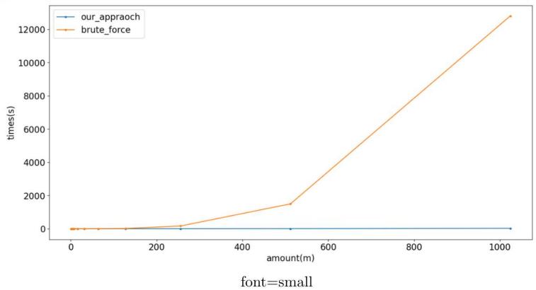
Figure 1. \( n \) v.s. time with the brute force and our approach

Note the brute force approach uses for loop instead of built-in @ operator when computing vector matrix multiplication. We did this on purpose since @ operation is optimized and does not reflect the underlying time complexity of matrix multiplication. Of course, we avoid using @ operator in our optimized algorithm for fairness.

We then plot the running time of our method against the recovery time complexity.

Figure 2. \( n \) v.s. time with the time complexity and our approach

6. Conclusion and Future Works

We proposed an efficient recovery algorithm that utilizes the math property of Lindström’s construction. The algorithm is much faster than the brute force approach, and its running time with our implementation is on par with what we conclude in theory.

For open problems, we note that we haven’t explored any lower bounds yet - it would be an interesting question to see if there is any non-trivial lower bound and how large the gap is with our current upper bound. One concrete question is, is \( Ω(mn) \) the lower bound? Do we have to compute most of \( {λ_{r}}D \) for every \( r \) ? Can we possibly do better?

References

[1]. Lindström, B. (1971). On Möbius functions and a problem in combinatorial number theory. Canadian Mathematical Bulletin, 14(4):513-516.
[2]. Cantor, D. G. and Mills, W. H. (1964). Determination of a subset from certain combinatorial properties.
[3]. Bshouty, N. H. (2009). Optimal algorithms for the coin weighing problem with a spring scale. In COLT, volume 2009, page 82.
[4]. Bose, R. C. and Ray-Chaudhuri, D. K. (1960). On A class of error correcting binary group codes. Inf. Control., 3(1):68-79.
[5]. Gebhard, O., Hahn-Klimroth, M., Kaaser, D., and Loick, P. (2019). Quantitative group testing in the sublinear regime. CoRR, abs/1905.01458.
[6]. Karimi, E., Kazemi, F., Heidarzadeh, A., Narayanan, K. R., and Sprintson, A. (2019).
Cite this article
Wang,H. (2024). The recovery time complexity of a coin weighing algorithm. Theoretical and Natural Science,30,195-204.
Data availability
The datasets used and/or analyzed during the current study will be available from the authors upon reasonable request.
Disclaimer/Publisher's Note
The statements, opinions and data contained in all publications are solely those of the individual author(s) and contributor(s) and not of EWA Publishing and/or the editor(s). EWA Publishing and/or the editor(s) disclaim responsibility for any injury to people or property resulting from any ideas, methods, instructions or products referred to in the content.
About volume
Volume title: Proceedings of the 3rd International Conference on Computing Innovation and Applied Physics
© 2024 by the author(s). Licensee EWA Publishing, Oxford, UK. This article is an open access article distributed under the terms and
conditions of the Creative Commons Attribution (CC BY) license. Authors who
publish this series agree to the following terms:
1. Authors retain copyright and grant the series right of first publication with the work simultaneously licensed under a Creative Commons
Attribution License that allows others to share the work with an acknowledgment of the work's authorship and initial publication in this
series.
2. Authors are able to enter into separate, additional contractual arrangements for the non-exclusive distribution of the series's published
version of the work (e.g., post it to an institutional repository or publish it in a book), with an acknowledgment of its initial
publication in this series.
3. Authors are permitted and encouraged to post their work online (e.g., in institutional repositories or on their website) prior to and
during the submission process, as it can lead to productive exchanges, as well as earlier and greater citation of published work (See
Open access policy for details).