1.Introduction

Synchronization, as a concept and observable phenomenon, spans a vast spectrum of disciplines. From the exact sciences like physics [1,2], biology [3,4], and chemistry to the intricate realms of music [5], economics, and art, its influence remains profound. As we delve into understanding the intricacies of the world's inherent order, synchronization emerges as a foundational cornerstone, offering pivotal insights into the structured rhythms of existence.

The fascination with synchronization can be traced back to the observations of the Dutch polymath, Huygens [6]. He discerned that paired pendulums, irrespective of their starting positions, would eventually oscillate in tandem, achieving congruent frequencies but with opposing phases. Modern studies, like those by Wiesenfeld [7], posited that for reverse synchronization to occur, pendulums must have a lower mass and exhibit minimal frequency disparities. Pantaleone's research [8] elucidated how increased friction between tabletops and pendulum bases made the observation of reverse synchronization more prevalent. Further, insights from Nijmeijer [9] indicated that systems with smaller beam masses were predisposed towards isochronous synchronization, while those with heavier crossbeams veered towards a reverse synchronization state.

Our research seeks to augment this body of knowledge by marrying experimental observations with numerical simulations. By blending analytical modelling with semi-empirical numerical modeling, we aim to delve into the nuances of metronome synchronization. This exploration is not just foundational but also navigates the intricate effects of platform mass, friction, and coupling strength on the phenomenon.

Section 2 anchors itself in the empirical realm, focusing on metronome synchronization. Through the lenses of image processing and audio frequency recognition techniques, the effects of platform friction on synchronization are meticulously analyzed. In Section 3, we transition to the theoretical domain, constructing a physical model that encapsulates two metronomes on a flat plate. The fourth-order Runge-Kutta method offers the computational prowess for our simulations, examining the nuanced relationship between friction and synchronization. Finally, Section 4 integrates the Kuramoto model, a revered semi-empirical methodology. Here, the synchronization dynamics of metronomes are simulated, with a distinct emphasis on the role of coupling strength in modulating synchronization behaviors.

2.Synchronization Investigation of Metronomes on an Oscillating Platform

2.1.Test configuration

A comprehensive experimental study was undertaken to elucidate the synchronization phenomena of metronomes under variable conditions. A typical apparatus comprised two mechanical metronomes, sourced from the renowned German manufacturer Wintner, with operational frequency ranges spanning from 40 bpm to 208 bpm. (as illustrated in Figure 1). Remark that this is just a demonstration on how the metronomes is placed on the rolling platform. In the following section, different numbers of the metronomes may be used.

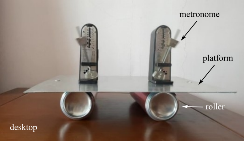
Figure 1. A typical experimental setup

In the isotropic synchronization experiment, a rigid board was utilized as the base, upon which two cylindrical cans were positioned. An aluminum plate was subsequently laid atop these cans, serving as the platform for the metronomes. For image recording purposes, a camera, affixed to a tripod, was strategically aligned such that its optical axis remained parallel to the plane defined by the two metronomes. Following the initiation of the experiment, periodic photographic captures were secured to chronicle the transition of the metronomes from a state of asynchrony to one of complete synchrony.

The salient physical parameters incorporated into this investigation are elucidated in Table 1.

Table 1. Physical properties metronome experiment set-up

2.2.A Comprehensive Analysis of Individual Metronome Frequencies

The oscillation frequency of a metronome is determined by the distance between the slider and the center of rotation of the metronome's arm. Conventional commercial metronomes utilize a mechanical slider to modulate their tempo. However, frequency deviations can emerge even with identical slider positions. To quantify the frequency of individual metronomes, a sound analysis methodology was employed. Each metronomic tick generates a distinct sound waveform, as depicted in Figure 2 By identifying peaks within the recorded waveform, precise determination of a metronome's period was achieved, which facilitated subsequent frequency calculations.

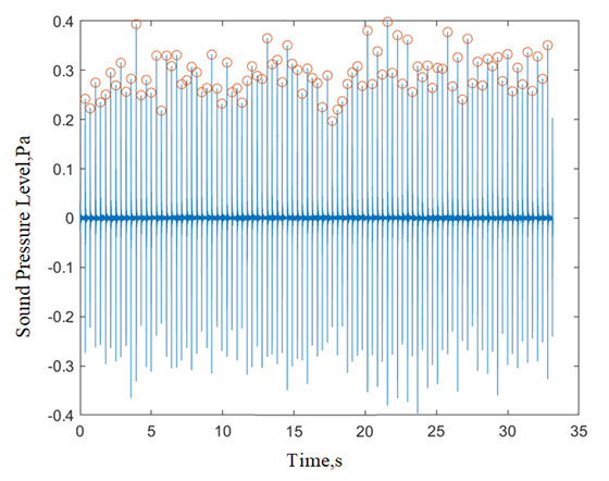
Figure 2. Time-domain representation of sound pressure for a prototypical metronome oscillation.

When choosing the metronomes, we identified the frequencies of different metronomes and chose two that have the most similar frequencies. When three metronomes were calibrated to an ostensible 128 bpm, experimental data (as illustrated in Figure 3) indicated true frequencies of 126 bpm, 125 bpm, and 124 bpm respectively. These frequencies consistently registered below the predefined value. Such discrepancies are believed to be due to the inherent imprecision of the mechanical slider mechanism.

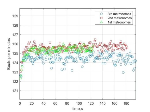
Figure 3. Frequency identification graphs for three distinct metronomes.

One metronome displayed a notably distinct oscillatory pattern compared to the others. To analyze this behavior, Tracker software was employed, enabling meticulous analysis of the pendulum's deflection angle over time.

During the investigation, three distinct trials were conducted. Each trial involved the release of a metronome and the video documentation of its oscillations. To ensure experimental consistency, the same initial phase was assigned to all metronomes. Upon stabilization of their oscillations, the angular deflection variation over a half-cycle was chronicled, as depicted in Figure 4.

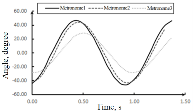
Figure 4. Temporal variation in metronome angular deflection.

From Figure 4, it is evident that not all metronomes converge to a uniform maximum deflection angle. Metronomes 1 and 2 exhibited proximate angular values, while metronome 3 deviated significantly. Such disparities might be attributed to manufacturing nuances, material variances, or differences in coil spring rigidity and damping. Despite the potential implications of these variances on synchronization experiments, the primary focus was on devising strategies to minimize the impact of these discrepancies on synchronization. As a result, subsequent studies exclusively incorporated metronomes 1 and 2 to ensure experimental consistency and reproducibility.

2.3.Effect of Friction on Metronome Synchronization

Friction plays a pivotal role in the study of metronome synchronization. Its magnitude and behavior can influence energy transfer, amplitude of oscillation, and the coupling dynamics between multiple metronomes. An understanding of how friction affects synchronization is crucial, as it provides insights into the mechanisms that either facilitate or inhibit coordinated oscillation. This section delves deeper into the intricate relationship between friction and the synchronization behavior of metronomes.

2.3.1.Influence of Desktop Material on Isotropic Release Metronome Synchronization. Experiments were conducted using two Aluminum cans as cylindrical rollers, placed on a horizontal acrylic platform. When two metronomes were released with identical initial phases in the same direction, they failed to synchronize, as demonstrated in Figure 5. Observations revealed that the metronomes remained out of phase and the platform exhibited minimal movement, resulting in an absence of synchronization.

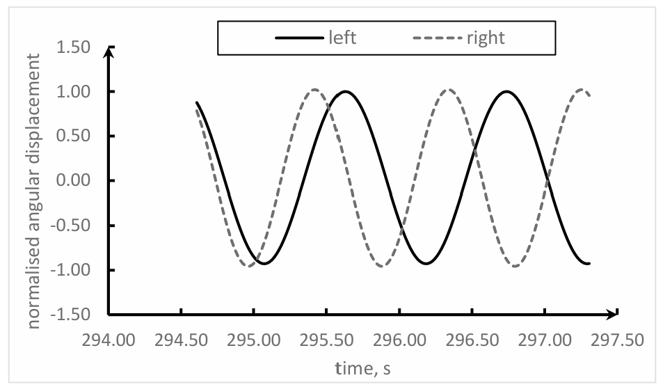
Figure 5. Desynchronization of two metronomes situated on a plastic horizontal platform.

Given the restricted motion of the platform, it was hypothesized that the coupling strength between the metronomes was intricately linked to the platform's motion. It was speculated that a significant friction coefficient, arising from the interaction of the platform material and the rollers, could consume vibrational energy, thus hindering the synchronization of the metronomes.

To further investigate this hypothesis, a wooden platform was used in place of the acrylic one, while all other conditions were retained. Following a brief phase of instability, the metronomes achieved a prolonged period of in-phase synchronization. The position of the metronome pendulum relative to a fixed point was measured at various intervals, from which the deflection angle was calculated. Figure 6 further attests to the isotropic synchronization phenomenon, underscoring the influence of the tabletop material on synchronization.

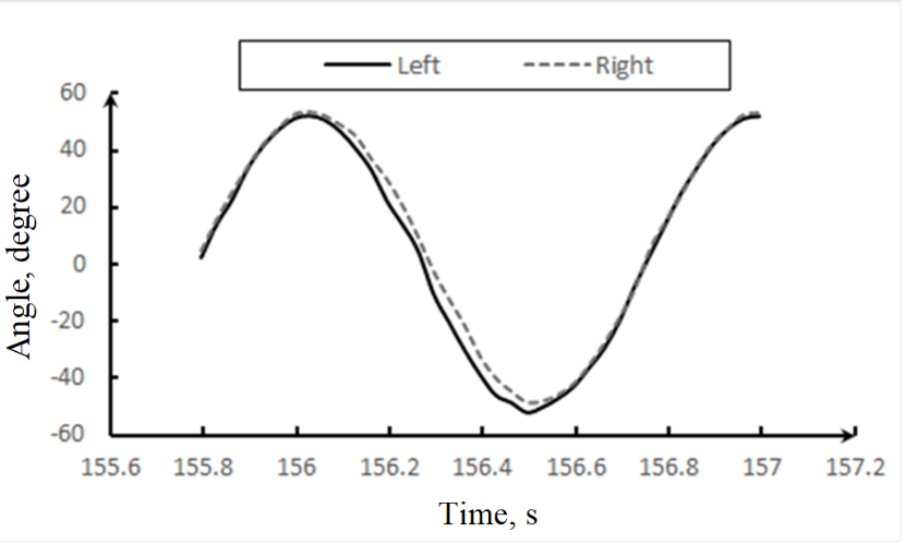
Figure 6. Time-domain representation of the deflection angle when subject to wooden desktop.

Literature [10] revealed that the kinetic friction coefficient between acrylic and aluminum stands at 0.6, while that between wood and aluminum is 0.2. This supported the hypothesis that in synchronization endeavors, when the material of the platform and the roller remains consistent, a decrease in friction between the two increases the likelihood of synchronization.

In summation, a lower friction coefficient bolsters the movement of the platform, which is pivotal for the coupling of the metronomes. By minimizing the energy dissipation of the platform, its displacement becomes more pronounced. This enhanced displacement facilitates a more efficient transfer of vibrational energy, resulting in the synchronization of the metronomes. This section suggests that synchronization largely hinges on the platform's capability to harmonize the frequencies and phases of both vibrational systems, culminating in synchronized oscillation.

2.3.2.Impact of Initial Phase on Metronome Synchronization. An intriguing aspect of metronome synchronization is the influence of the initial phase. It's hypothesized that the type of synchronization - isotropic or inverse - could be largely determined by the choice of initial phase, especially when the phase difference approximates 180 degrees.

Two metronomes were set with opposing initial phases and activated simultaneously. The temporal evolution of the deflection angles of the two metronome pendulums was examined. Analysis revealed that the oscillatory patterns of both metronomes exhibited symmetry relative to the time axis, thereby confirming the presence of inverse synchronization. Additionally, once the metronomes entered the state of reverse synchronization, the hitherto dynamically moving platform became static. This can be ascribed to the frictional forces applied by each metronome on the platform during reverse synchronization. These forces, equivalent in magnitude but opposite in direction, counteract each other, resulting in the cessation of the platform's movement.

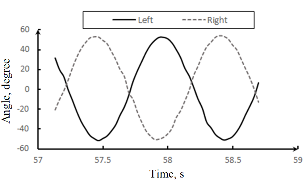
Figure 7. Time-domain representation of the deflection angle when subject to reversed initial phase.

2.3.3.Impact of Friction between cylinderical roller and platform on Synchronization Behavior. The interplay between friction and synchronization, as indicated in previous sections, hints at the critical role of the frictional interface between the roller and the platform. This section further investigates this relationship by manipulating the frictional properties via material variation for both the roller and the platform.

Initial experiments utilized a wooden horizontal tabletop, with the aluminum platform subsequently replaced by an acrylic plate. When two metronomes, with identical initial phases, were initiated, isotropic synchronization manifested after a given duration. The onset of this synchronization is depicted in Figure 8, showcasing minimal phase differences between the two metronomes.

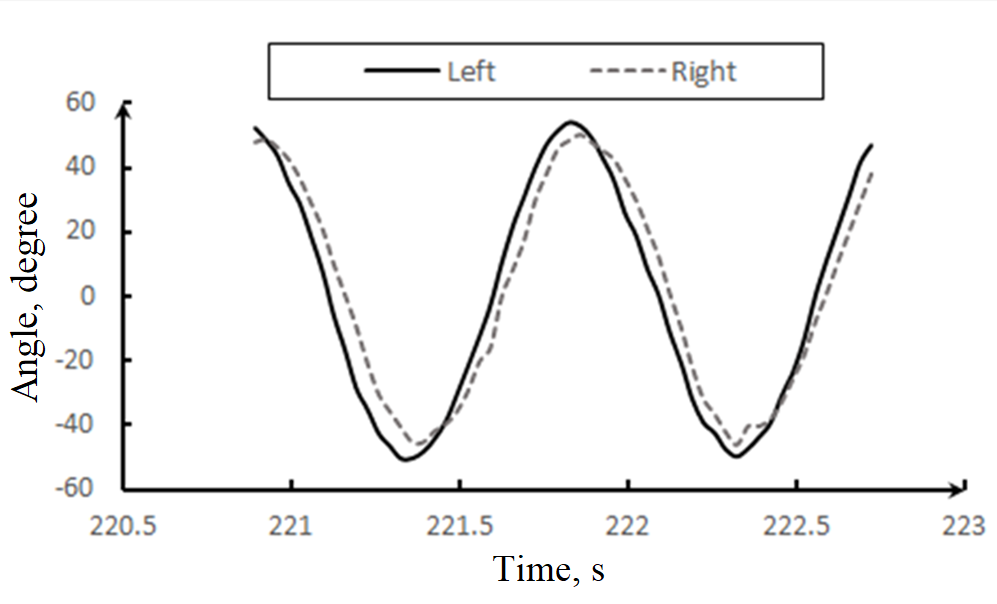
Figure 8. Time-domain representation of the deflection angle when subject to identical initial phase.

A subsequent set of experiments presented the metronomes with identical, yet reversed, initial phases. The results displayed a delay in achieving isotropic synchronization, particularly when compared to the first set (see Figure 7), with synchronization beginning around the 50th second. As Figure 9 shows, despite having opposing initial phases, the altered frictional dynamics produced a distinctive synchronization trajectory.

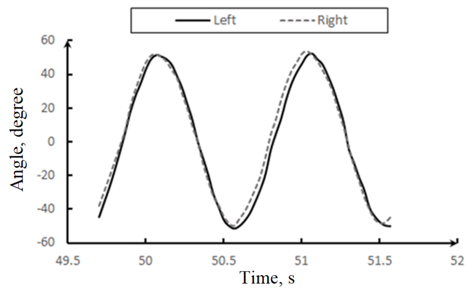
Figure 9. Time-domain representation of the deflection angle when subject to reversed initial phase.

Known coefficients of kinetic friction — 0.2 between an aluminum platform and roller, and 0.15 between an acrylic platform and roller — offer insights into these observations. [10] Specifically, the reduced frictional coefficient associated with the acrylic platform leads to a faster and more pronounced coupling effect, culminating in a quicker attainment of isotropic synchronization.

The dynamics can be summarized as follows: The periodic influence of friction on metronomes becomes more pronounced with a decrease in the frictional coefficient. As a result, the inherent phase differences between metronomes, even if they are slight, are more readily affected, prompting the plate to move. This movement, coupled with the decreased friction, accelerates the phase difference expansion. As the plate's vibration intensity grows, its influence on the pendulum intensifies, further altering the phase relation between the two pendulums. While the frictional dynamics are intricate, a lowered friction coefficient demonstrably accelerates the synchronization process, underpinning the crucial role friction plays in time-to-synchronization.

2.3.4.The Metronome Suppression Phenomenon. While earlier sections focused on synchronization behaviors under conditions of reduced friction, it is equally imperative to understand the dynamics under increased friction. In light of this, the experiments employed a pairing of acrylic plates and acrylic cylinders.

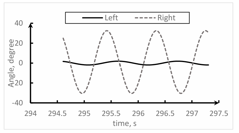
Figure 10. Visual representation of the eventual onset of the metronome suppression phenomenon.

Contrary to previously observed synchronization effects, a distinct "metronome suppression" phenomenon was evident in this experiment. This phenomenon emerges when one metronome experiences such a limited amplitude that it can't adequately power its escapement mechanism, rendering it ineffective. Conversely, the other metronome, albeit with a diminished amplitude, remains operational, leading to only marginal platform vibrations, hence termed as "metronome suppression". (as illustrated in Figure 10)

The underlying physics can be traced back to the dampening effects of friction on the metronomes' motion. Since both metronomes oscillate synchronously, friction impacts them equivalently. However, the frictional force isn't consistent. As a result, at certain intervals, one metronome might encounter heightened frictional forces, translating to a more pronounced energy depletion. Once this energy drain surpasses what's essential for escapement propulsion, the metronome's oscillation diminishes until halted. This halted metronome influences the plate minimally, subsequently reducing its amplitude. Nevertheless, the other metronome, being subject to a milder friction, retains its oscillatory motion and may even re-energize the previously halted metronome.

In essence, heightened friction can precipitate the metronome suppression effect – a multifaceted interplay of friction, escapement dynamics, and metronome interactions.

2.4.Summary

This section investigated the intricate dynamics of metronome behavior, blending experimental analysis with physical explanation. The initial focus was on individual metronomes' frequency characteristics and angular deflections. This progressed to a detailed data evaluation using Tracker, highlighting various factors (such as tabletop materials, initial phase, and platform-roller friction) that influence metronome synchronization. Significantly, this research provided insights into the "metronome suppression" phenomenon, shedding light on it for the first time.

The findings from this chapter lay a robust foundation for the subsequent sections. The forthcoming chapter is set to present a comprehensive model of the metronome structure, complemented by its motion equations derived from a physics perspective. The study will then venture into simulating the dual metronome behavior on a mobile tablet using numerical simulations, aiming to reveal the core factors underpinning metronome synchronization.

3.Physical modelling and numerical simulation of metronome synchronization

In the preceding section, frequency measurements of a single metronome and synchronization experiments with one or two metronomes placed on platform and tabletops of various materials were conducted. The experimental outcomes suggest that both the mass of the platform and the friction between the platform and the roller substantially affect the synchronization state of the metronomes. Yet, due to limitations in the experimental equipment, challenges arose in examining certain specific variables, notably the friction parameter between the flat plate and the cylinder. To address this, this chapter endeavors to develop a theoretical model of the metronome positioned on a flat platform, subsequently simulating this model using the fourth-order Lunger Kuta method. The objective behind this simulation is to undertake a thorough exploration of the circumstances under which metronome synchronization transpires and the elements that sway it. Through this analysis, a more holistic understanding and elucidation of the metronome synchronization phenomenon's nature and mechanism are sought, laying a robust theoretical groundwork for ensuing research.

3.1.Physical Structure of the Metronome

A metronome is best conceptualized as a distinct type of mono-pendulum structure, equipped with two suspended mass blocks. The upper mass can be vertically displaced at will, whereas the lower mass remains stationary. Modulating the position of the upper mass permits alteration of the pendulum's effective length, subsequently adjusting the metronome's vibrational natural frequency. It's imperative to underscore that if a metronome were purely a passive entity, influenced solely by air resistance and internal damping, its amplitude would gradually diminish until it came to a halt. The pivotal role in sustaining the metronome's continuous vibration is played by the Escapement Mechanism.

This Escapement Mechanism can be dissected into four principal moments, as depicted in Figure 11. In the initial moment, the green gear engages with the red escapement fork, instantaneously imposing a clockwise torque on the escapement fork. This torque prompts the escapement fork to persistently rotate counterclockwise, although its angular velocity sees a gradual reduction. In the subsequent moment, the escapement fork achieves its counterclockwise rotation zenith, at which juncture the pink gear engages with the fork. Now, the escapement fork, aligned with its rotation center, ceases to exert torque on the system, rendering it dynamically neutral. At the third moment, the system reverts to a state reminiscent of the initial moment, and the cycle ensues.

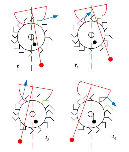
Figure 11. Schematic Illustration of the Escapement Mechanism's Operation.

3.2.Dynamics of Metronomes on a moving platform

To streamline the analysis, the dynamic properties of a metronome placed on a flat plate with rollers were first investigated, as depicted in Figure 12.

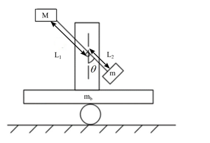
Figure 12. Schematic Diagram of a Single Metronome on a Flat Plate with Friction.

The motion equation for the metronomes is as follows:

\( J\ddot{θ}+(M{L_{1}}+m{L_{2}})gsin{θ}+{m_{b}}cos{θ}\ddot{x}+{ξ_{1}}{\dot{θ}_{1}}={f_{1}} \)(1)

where\( \ddot{θ} \)represents angular acceleration and\( J \), the moment of inertia is as follows:

\( J=m{R^{2}} \)(2)

The term\( {ξ_{1}}{\dot{θ}_{1}} \) represents the damping force of the oscillatory decay. The excitation force,\( f \), exerted by the escapement on the pendulum at a given moment, is represented as follows:

\( fδ(t-{t_{*}})=\begin{cases}\begin{matrix}0 & t≠{t_{*}} \\ f & t={t_{*}} \\ \end{matrix}\end{cases} \)(3)

This denotes the moment when the escapement provides the pendulum with an excitation force.

The movement of the platform influences the metronome throughout the system’s motion. The reaction force of the platform on the metronome is defined as\( {F_{base}}r cos \). According to Newton’s third law, this reaction force is antiparallel but equal in magnitude to the inertial force on the flat plate. This reaction force is therefore formulated as:

\( {F_{base}}={m_{b}}\ddot{x} \)(4)

where\( {m_{b}} \)is the mass of the plate.

Next, a separate force analysis was conducted on the flat plate (as illustrated in Figure 13):

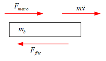
Figure 13. Schematic Representation of the Forces on a Flat Plate.

Here, the reaction force,\( {F_{metro}} \), of the metronome displacement on the flat plate is initially analyzed. This reaction force is equal to the inertial force of the metronome pendulum in the direction of translation, according to Newton's third law. To derive this inertial force, the angular displacement of the metronome is converted to displacement in the direction of translational motion of the flat plate, denoted as\( {L_{2}}sin{θ} \). Then, by performing double integration concerning time, its acceleration in the direction of the translational motion of the flat plate is obtained and denoted as\( {L_{2}}(\ddot{θ}cos{θ}-{\dot{θ}^{2}}sin{θ}) \). This displacement is then multiplied by its mass to derive this inertial force. The equation for the advection of the flat plate is as follows, according to Newton’s second law:

\( {m_{b}}\ddot{x}+(M{L_{1}}+{mL_{2}})(\ddot{θ}cos{θ}-{\dot{θ}^{2}}sin{θ})+{F_{1}}=0 \)(5)

Post-analysis of the mechanical equilibrium of a single metronome, this chapter further explores the mechanical equilibrium of two metronomes on a moving flat plate. Following a similar force analysis of a single metronome on a flat plate, the motion equations for two metronomes on a flat plate can be derived:

Here,\( F \)represents the friction force,\( μ \)is the coefficient of sliding friction, and\( {f_{1}} \)and\( {f_{2}} \)denote the excitation force for two metronomes, respectively.

3.3.Introduction to numerical simulation methods

The simulation of the metronome presented unique challenges. Notably, the abrupt changes in metronome excitation, caused by the escapement structure, appeared as sudden spikes. These sudden increases resulted in angles that exhibited a slope tending towards positive infinity at specific points. Directly applying the Lunger Kuta method to such a differential equation would not be feasible due to these instantaneous anomalies [11].

To address this challenge, a segmented approach was taken for the vibration period of the metronome. This approach entailed discretizing angles and angular velocities within each vibration cycle. This ensured that the sudden excitation changes from the escapement mechanism could be efficiently managed. For clarity, a complete vibration cycle was broken down into five distinct phases (refer to Figure 14):

•Phase 1 (0 ≤ t < T₁): In this phase, the metronome operates without any external excitations affecting its swing.

•Phase 2 (T₁ ≤ t < T₁ + δ₁): This short duration witnesses the metronome being affected by an external excitation, leading to a sharp rise in its angular velocity. The angular velocity's rate of change is notably high during this phase.

•Phase 3 (T₁ +δ₁ ≤ t < T₂): Post the sudden excitation, the metronome resumes its unimpeded swing until the next excitation occurs.

•Phase 4 (T₂ ≤ t < T₂ + δ₂): Similar to Phase 2, but here the metronome faces a reverse excitation, leading to a sharp drop in its angular velocity. Once again, the rate of change of angular velocity is considerably high.

•Phase 5 (T₂ + δ₂ ≤ t < T_period): The metronome completes its vibration cycle by oscillating freely post the last excitation.

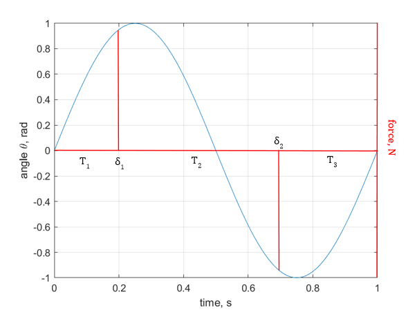
Figure 14. Variation of metronome deflection angle against time under excitation influences.

By adopting this phased approach, the numerical solution can effectively manage rapid changes in angular velocity, ensuring the stability of results.

The challenge of integrating the metronome's behavior with friction arises due to the inherent directionality of frictional forces. Friction always acts in a direction opposite to the motion of the object it affects. In the context of our numerical simulations, the frictional force would act opposite to the velocity of the platform on which the metronome rests. This directionality must be appropriately captured to ensure accurate simulation results. Figure 15 provides a schematic representation of how the simulation progresses, incorporating the ever-present frictional forces that oppose the platform's motion.

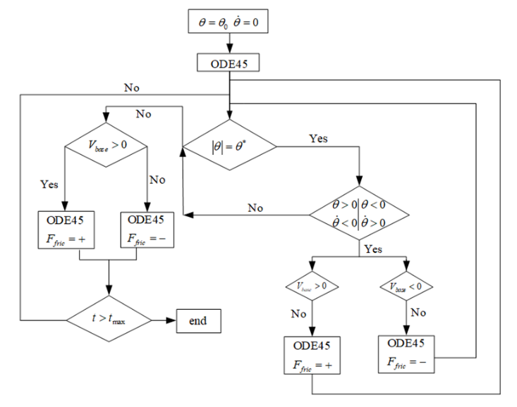
Figure 15. Flowchart depicting the numerical simulation of a metronome on a frictional flat plate.

3.4.Simulation and observation

For the simulation, the physical parameters of the metronome and the platform were as listed in Table 2.

Table 2. Physical parameters of metronome and plate.

According to the simulation results (see Figure 16), the angular displacements of the two metronomes showed contrasting patterns, implying that the metronomes exhibited reverse synchronization.

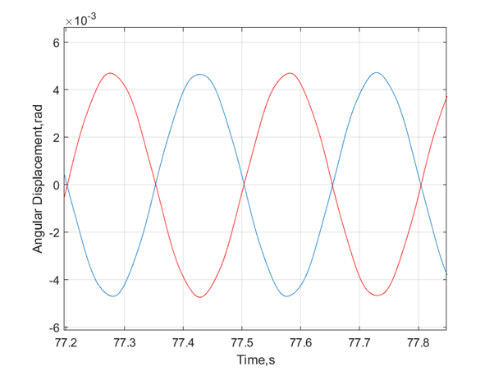
Figure 16. Angular displacement for two reverse-synchronized metronomes on a frictional moving platform of 1 kg (frictional coefficient is\( 6.4×{10^{-4}} \))

To better understand the influence of the friction coefficient on synchronization, we adjusted the coefficient for another numerical simulation. Keeping the mass of the weight at 0.5 kg, we observed that due to the lower friction coefficient, the system's energy dissipated more slowly. This enabled the metronome's excitation mechanism to sustain vibration for 100 seconds. (refer to Figure 17)

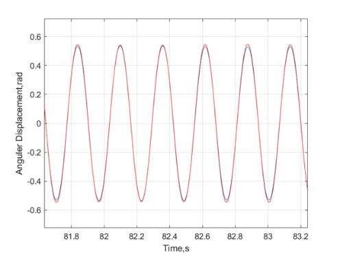
Figure 17. Angular displacement for two isotropic synchronized metronomes on a frictional moving plate of 1 kg (friction coefficient is\( 6.4×{10^{-6}} \))

Furthermore, to deeply investigate the weight's impact on coupling strength, we adjusted the weight's mass to both 0.25 kg and 1.5 kg in separate simulations, while keeping the friction coefficient consistent. Observations indicated diverse synchronization behaviors, with reverse synchronization appearing prominently when the mass was adjusted (referring to Figure 18).

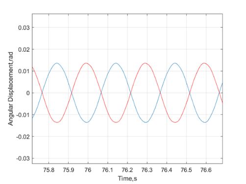
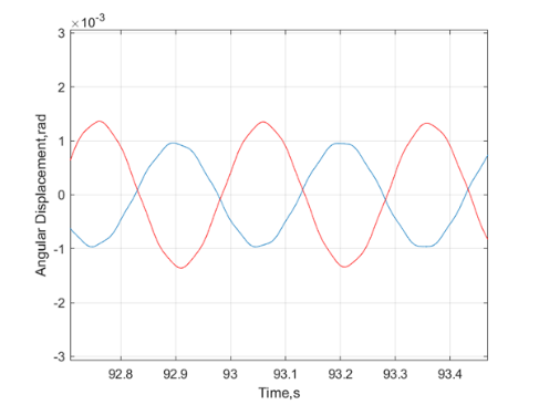
Figure 18. Angular displacement for two isotropic synchronized metronomes on a frictional moving plate of (a) 0.25 kg and (b) 1.5 kg (friction coefficient is\( 6.4×{10^{-6}} \))

3.5.Summary

This section delivered a comprehensive discussion on the metronome's physical structure, further delving into modeling and numerical simulation of its dynamics both as a singular entity and in pairs, under different conditions. By contrasting the metronome's behavior on a damped flat plate against one with friction, we affirmed that friction presents a more accurate depiction of the system's dynamic behavior. Consequently, in subsequent studies, when considering the synchronization of two metronomes, we integrated friction into the system's dynamic model. We also examined how both the coefficient of friction and the mass of additional weight impacted the synchronization phenomenon.

While the physical modeling enriched our understanding, the next chapter will introduce the Kuramoto model, addressing the complexity of our current model and the challenges in acquiring certain experimental parameters. This new model, being more concise, is expected to elucidate the effects of coupling strength on synchronization behavior more efficiently.

4.Semi-empirical model: Kuramoto approach

This section underscores the challenges of traditional physical modeling, notably the extensive simulation times and the hurdles in acquiring precise system parameters. Additionally, such conventional methods often cannot directly quantify the coupling strength, nor do they provide a clear demarcation between isotropic and inverse synchronization. To navigate these issues and provide a more lucid analysis of how coupling strength impacts synchronization, the Kuramoto model is introduced. By employing this streamlined approach for numerical simulations, the analysis becomes more focused, elucidating the relationship between coupling strength and the synchronization phenomenon.

4.1.Kuramoto model for harmonic oscillator coupling

The Kuramoto model is a renowned mathematical model employed to characterize the dynamics of a system of coupled oscillators. [12] Recognized as a semi-empirical model, it encompasses\( i \)coupled oscillators. The governing equation for each oscillator is described as:

\( \frac{d{θ_{1}}}{dt}={ω_{i}}+λ\sum _{j=1}^{N}sin{({θ_{j}}-{θ_{i}})},i=1,…,N \)(7)

Here,\( λ \)represents the coupling strength,\( {ω_{i}} \)signifies the intrinsic frequency, and\( {θ_{i}} \)denotes the phase of the\( i \) ^th oscillator.

In the case of two mutually coupled oscillators, the Kuramoto model simplifies to:

\( \frac{\frac{d{θ_{1}}}{dt}={ω_{1}}+λsin{({θ_{2}}-{θ_{1}})}}{\frac{d{θ_{2}}}{dt}={ω_{2}}+λsin{({θ_{1}}-{θ_{2}})}}\ \ \ (8) \)

These equations succinctly encapsulate the interaction dynamics between the two oscillators and the evolution of synchronization.

The term\( sin{({θ_{j}}-{θ_{i}})} \)captures the influence of the phase differential between oscillator\( i \)and\( j \)on the phase change rate of oscillator\( i \). When the phase difference nears zero,\( \dot{{θ_{i}}} \)approximates\( {ω_{i}} \), signifying that oscillator\( i \)maintains a phase change rate closely tied to its

intrinsic frequency. Yet, when the phase difference is near\( π \), the influence becomes paramount, thus leading the phase of oscillator\( i \)to either accelerate or decelerate, ensuring phase synchronization between\( i \)and\( j \).

By designating the phase of the first oscillator as our reference, and with\( λ \)>0 oscillators experience contrasting coupling effects. This results in one oscillator having an accelerated phase compared to the other, driving them towards synchronization. However, for\( λ \)<0, the two oscillators are inclined towards anti-synchronization, with their phases moving in opposing directions.

4.1.1.Order Parameter. A critical metric when determining the synchronization of resonators within a system is the Order Parameter. This parameter serves as an indicator of the phase distribution among the resonators, primarily highlighting their temporal alignment.

For the Kuramoto model, the order parameter is mathematically defined as:

\( Z=R{e^{iψ}}=\frac{1}{N}\sum _{j=1}^{N}{e^{{iθ_{j}}}} \)(9)

Where:

Z is the order parameter, represented as a complex number with modulus constrained to 1. R is the amplitude, elucidating the degree of synchronization. ψ is the phase, depicting the average phase of the oscillators. N is the number of oscillators, and θ_j is the phase of the j^th oscillator.

An intuitive way to grasp the physical significance of the order parameter is to envision the phase of each oscillator as a unit vector within the complex plane. In this representation, every oscillator's phase corresponds to a vector on the unit circle. Computing the order parameter is equivalent to averaging these unit vectors.

In conditions where the system manifests reverse synchronization, the vectors corresponding to the oscillator phases neutralize each other. This results in a diminished magnitude of the average vector, with R=0 symbolizing complete disorder. Conversely, in a fully synchronized state, most vectors align in a common direction, leading to a higher average vector magnitude, signified by R=1. For intermediary synchronization states, the value of R lies between 0 and 1.

4.1.2.Case study of asynchronous and synchronous phenomena. For the initial setup, parameters were assigned to the two resonators with initial phases as\( {θ_{1}} \)=0.1 rad,\( {θ_{2}} \)=3.8 rad, coupling strength as\( λ \)=0.5, eigenfrequency as\( {ω_{1}} \)=2.0 rad/s,\( {ω_{2}} \)=4.2 rad/s, and a time grid accuracy of\( Δt \)=0.01. Figure 19 displays an oscillation of the order parameter between 0 and 1, signifying the system's lack of synchronization.

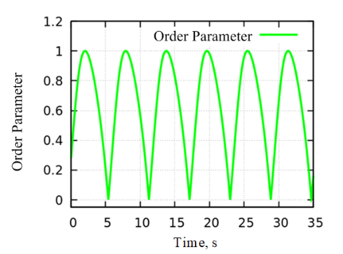
Figure 19. Time-domain diagram of order parameters (unsynchronized state).

The evolution of phase with time, presented in Figure 20, further verifies the absence of synchronization between the two resonators.

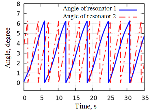
Figure 20. Phase change versus time of two resonators that are not synchronized.

Upon adjusting parameters, with initial phases set to\( {θ_{1}} \)=0.1 rad,\( {θ_{2}} \)=3.8 rad, coupling strength to\( λ \)=0.8, eigenfrequency to\( {ω_{1}} \)=12.0 rad/s,\( {ω_{2}} \)=12.2 rad/s, and the same time grid accuracy retained, the order parameter's progression is evident in Figure 21. It consistently rises until it nears 1, indicating system synchronization.

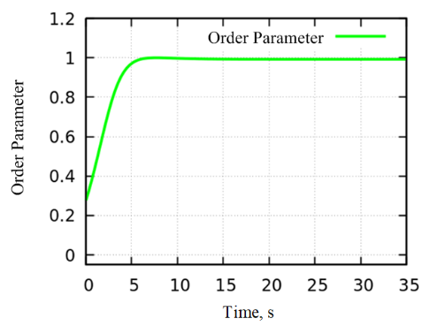
Figure 21. Time-domain diagram of order parameters (synchronized state).

The synchronization of the two resonators is further elucidated by Figure 22, which delineates their phase transitions over time.

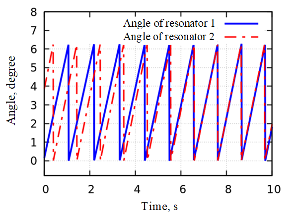
Figure 22. Time evolution of phase difference for two synchronized resonators.

4.1.3.Discussion. The numerical findings yield a crucial insight. Despite reaching synchronization, the order parameter does not attain a value of exactly 1. Rather, it hovers close to this number. This nuanced observation underscores the presence of slight disparities in the intrinsic frequencies of the two resonators. Additionally, the influence of platform coupling implies that these intrinsic frequencies aren't static but exhibit temporal fluctuations.

In the dynamics of synchronization, these disparities lead to alternating dominance between the two resonators. Instead of a firm, invariable connection that might be seen with perfect synchronization, a more adaptable, malleable coupling is observed. Such an interaction mirrors the characteristic synchronization patterns witnessed in the experimental observations from the preceding chapter and the numerical simulations discussed in this section.

This reinforces the notion that the real-world phenomena of synchronization often entail subtleties and complexities that might not be entirely captured by an idealized model. However, the Kuramoto approach provides a valuable framework for understanding and quantifying the major dynamics at play.

4.2.Observations from Large-scale Simulation

Expanding on the basic premise of two resonator synchronization, the simulation of a system with a hundred resonators was conducted. This not only tested the scalability of the observed synchronization behaviors but also furthered the exploration into the collective dynamics of larger ensembles.

For this scenario, the initial conditions were randomized: phases were drawn from a uniform distribution spanning 0 to 2π, while the eigenfrequencies were chosen randomly from a tight range between 12 and 12.05 rad/s. This narrow range ensures that all the resonators are close in their innate frequencies, though not identical. The other parameters, such as coupling strength and time grid accuracy, were held constant for the simulation.

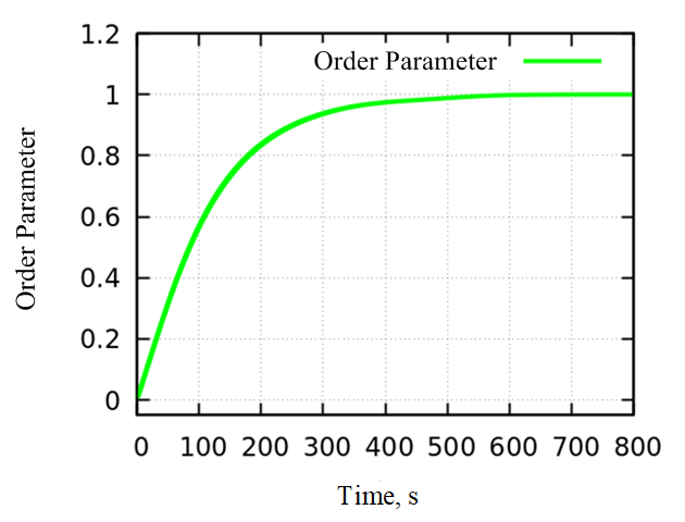
Figure 23. Time-domain diagram of order parameters (100 resonators).

The time-domain plot of the order parameter, depicted in Figure 23, demonstrates a progression towards synchronization. Initially, the order parameter is relatively low, reflecting the random initial conditions of the resonators. As time progresses, the order parameter escalates, tending towards 1, signaling that the system is moving towards complete synchronization.

The visualization of phase changes in real-time, shown in Figure 24, offers a granular perspective on the trajectory of each resonator. The transition from a disordered and random phase state to a more coherent, aligned state is evident. By the end of the simulation, the phases of the resonators are nearly identical, though not perfectly so. This closely aligned but slightly disparate phase alignment is consistent with the findings from the two-resonator simulations. It emphasizes the presence of a soft or flexible synchronization, rather than a rigid one.

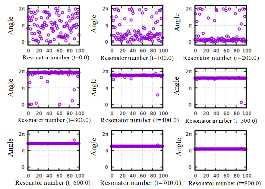
Figure 24. Simulation of the phase of one hundred resonators from completely random to gradually converging to synchronization.

In conclusion, the extrapolation from two resonators to a hundred resonators validates the robustness of the observed synchronization behaviors. The intricacies and slight variations in phases, even when synchronized, emphasize the dynamism inherent in real-world systems. The findings underscore the significance of considering both global metrics like the order parameter and local dynamics, such as individual phase trajectories, to gain a holistic understanding of synchronization in large oscillator ensembles.

4.3.Implications and Observations

In exploring the dynamics of synchronization, this section utilized numerical simulations to delve into the influence of frequency differences between two resonators on the required coupling strength for synchronization. For this, two distinct experiments were conducted. Initially, with an intrinsic frequency of one resonator set at 10 rad/s, the frequency of its counterpart was varied from 10 to 14 rad/s at increments of 0.2 rad/s. In a subsequent experiment, the initial resonator's frequency was fixed at 18 rad/s while the other ranged from 18.0 to 22.0 rad/s in 0.4 rad/s intervals. Upon analyzing the data, it emerged that synchronization is more easily achieved with minimal coupling strength when the resonators’ frequencies are closely matched. As the frequency disparity grows, the coupling strength necessary for synchronization increases proportionally. This is depicted in Figure 25.

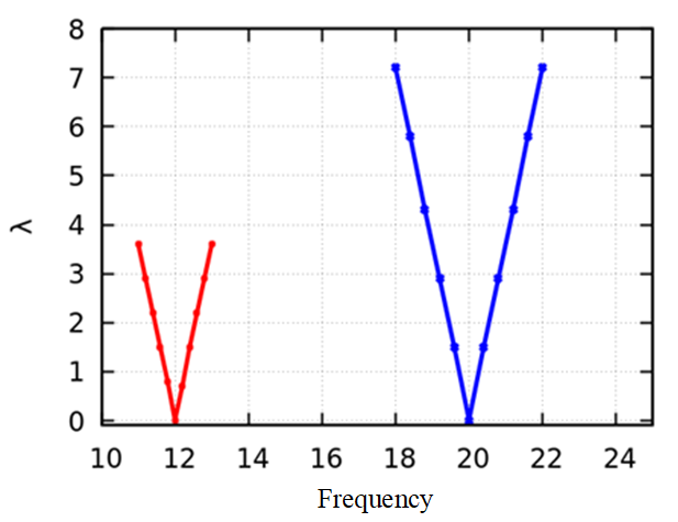
Figure 25. Correlation between synchronization and coupling strength in numerical simulations.

It is paramount to recognize that the Kuramoto model, despite its utility in these simulations, remains a mathematical construct. The observed symmetrical patterns, while theoretically sound, might not completely represent physical real-world scenarios. Hence, real experimental data is indispensable. The intricate interplay between various physical parameters and coupling strengths in real situations often surpasses the capabilities of the semi-empirical model. In essence, while the Kuramoto model aids in understanding synchronization, comprehensive knowledge necessitates an amalgamation of theory and empirical testing.

4.4.Summary

This chapter explored the intricate behavior of resonator coupling using the Kuramoto model. An initial focus was directed towards understanding the isotropic synchronization behaviors, with the order parameter's time-dependent variation serving as a key observation metric. Extending the study from a dual-resonator scenario, synchronization under multi-resonator coupling was simulated, involving up to 100 resonators.

A pivotal investigation was carried out on the effect of frequency disparities between two resonators on the required coupling strength for synchronization. Results indicated that as the intrinsic frequencies of resonators drew closer, the synchronization was achieved with relatively lower coupling strengths.

It's imperative to recognize the limitations of the Kuramoto model, as real-world complexities in synchronization phenomena might not be entirely encapsulated within this model. Future endeavors in this research domain should consider a hybrid approach, intertwining the insights from the Kuramoto model with empirical experiments, to yield a more holistic understanding of the underlying relationships between physical parameters and synchronization.

5.Conclusion

This research melds the mathematical modeling with the explorative insights of semi-empirical approaches, delivering a comprehensive understanding of mechanical metronome synchronization dynamics.

Our journey commenced with an in-depth characterization of individual metronomes, focusing on their distinct frequency and deflection angle behaviors. Utilizing the Tracker software, we delved into the intricacies of synchronization. This empirical endeavor provided insights into factors such as desktop material, the impact of initial phase differences, and the pivotal role of friction between the roller and platform. One particularly intriguing discovery was the metronome suppression phenomenon, a topic ripe for future investigation.

In terms of theoretical contributions, our mathematical model, constructed on foundational physical laws, provided a solid framework to unravel synchronization behaviors. We numerically solved the differential equations derived from the model, employing 4th order Newton-Raphson method using MATLAB, to further our understanding of the synchronization phenomenon.

Complementing our mathematical pursuits, the Kuramoto model, a semi-empirical tool, facilitated insights into the effects of coupling strength on synchronization. Through a battery of simulations, we were able to discern synchronization behaviors across a spectrum of resonator frequencies. A critical takeaway was the inverse relationship between resonator frequency proximity and the required coupling strength for effective synchronization.

Looking ahead, we plan to refine and further validate our mathematical model. Key focal points will include the determination of metronome escapement excitation angles, in-depth quantification of both escapement excitation and damping forces, and a deeper exploration of the frictional dynamics involved. Empirical studies will augment these endeavors, examining synchronization under a myriad of physical conditions, linking coupling strength to plate displacements, and mapping the relationships between coupling strength and various influential parameters.

References

[1]. Tajima H, Funo K, Superconducting-like Heat Current: Effective Cancellation of Current-Dissipation Trade-Off by Quantum Coherence[J], Physical Review Letters, 2021, 127(19): 190604.
[2]. Ticos C, Rosa E, Pardo W, et al., Experimental real-time phase synchronization of a paced chaotic plasma discharge[J], Physical Review Letters, 2000, 85(14): 2929.
[3]. Ramirez J, Nijmeijer H, The secret of the synchronized pendulums[J], Physics World, 2020, 33(1): 36.
[4]. Buck J, Buck E, Mechanism of Rhythmic Synchronous Flashing of Fireflies: Fireflies of Southeast Asia may use anticipatory time-measuring in synchronizing their flashing[J], Science, 1968, 159(3821): 1319-1327.
[5]. Rayleigh J W S B. The theory of sound[M]. Macmillan, 1896.
[6]. Huygens Ch, Œuvres complètes[M], Swets & Zeitlinger B. V., Amsterdam, 1967.
[7]. Bennett M, Schatz M F, Rockwood H, et al. Huygens's clocks[J]. Proceedings of the Royal Society of London. Series A: Mathematical, Physical and Engineering Sciences, 2002, 458(2019): 563-579.
[8]. Pantaleone J. Synchronization of metronomes[J]. American Journal of Physics, 2002, 70(10): 992-1000.
[9]. Kuznetsov N V, Leonov G A, Nijmeijer H, et al. Synchronization of two metronomes[C]//PSYCO. 2007: 49-52.
[10]. Hutchings I, Shipway P. Tribology: friction and wear of engineering materials[M]. Butterworth-heinemann, 2017.
[11]. Cartwright J H E, Piro O. The dynamics of Runge–Kutta methods[J]. International Journal of Bifurcation and Chaos, 1992, 2(03): 427-449.
[12]. Acebrón J A, Bonilla L L, Vicente C J P, et al. The Kuramoto model: A simple paradigm for synchronization phenomena[J]. Reviews of modern physics, 2005, 77(1): 137.
Cite this article
Wu,W. (2024). Metronome synchronization in the presence of friction. Theoretical and Natural Science,31,19-40.
Data availability
The datasets used and/or analyzed during the current study will be available from the authors upon reasonable request.
Disclaimer/Publisher's Note
The statements, opinions and data contained in all publications are solely those of the individual author(s) and contributor(s) and not of EWA Publishing and/or the editor(s). EWA Publishing and/or the editor(s) disclaim responsibility for any injury to people or property resulting from any ideas, methods, instructions or products referred to in the content.
About volume
Volume title: Proceedings of the 3rd International Conference on Computing Innovation and Applied Physics
© 2024 by the author(s). Licensee EWA Publishing, Oxford, UK. This article is an open access article distributed under the terms and
conditions of the Creative Commons Attribution (CC BY) license. Authors who
publish this series agree to the following terms:
1. Authors retain copyright and grant the series right of first publication with the work simultaneously licensed under a Creative Commons
Attribution License that allows others to share the work with an acknowledgment of the work's authorship and initial publication in this
series.
2. Authors are able to enter into separate, additional contractual arrangements for the non-exclusive distribution of the series's published
version of the work (e.g., post it to an institutional repository or publish it in a book), with an acknowledgment of its initial
publication in this series.
3. Authors are permitted and encouraged to post their work online (e.g., in institutional repositories or on their website) prior to and
during the submission process, as it can lead to productive exchanges, as well as earlier and greater citation of published work (See
Open access policy for details).