1. Introduction

In recent years, the trend of rising housing prices has been continuously observed. The positive effects of housing policies will largely impact various aspects of people’s lives, such as marriage [1]. For those who have just entered the workforce, renting remains a relatively affordable way to accumulate capital for purchasing a house. Similarly, for individuals with temporary accommodation needs in a city where they do not plan to settle permanently, renting is a reasonable option. Compared to purchasing property, renting offers lower costs while still providing the advantages of location. However, rental properties vary widely in quality and level of renovation. The rental price of a property is influenced by numerous factors, and understanding which factors contribute more significantly to the rental price is of great research interest.

Linear regression models are often employed as crucial tools to study the influence of certain factors on the subject of research. Indeed, numerous studies are conducted based on linear regression. Akakuru, Adakwa, and Ikoro collected data from 40 surface water samples and conducted research using multivariate linear regression (MLR) models to predict groundwater quality parameters such as ecological risk index (ERI), pollution load index (PLI), metal pollution index (MPI), Nemerow pollution index (NPI), and geoaccumulation index (Igeo) [2]. Khandaskar et al. utilized linear regression models to develop prediction systems for housing prices and rents [3]. These studies ensure the rationality of analyzing and predicting house rents using linear regression models.

It has a remarkable effectiveness of linear regression in price prediction. Wei et al. showed that many factors influence rental prices [4]. Subsequently, there have been numerous studies using linear regression models to investigate factors influencing house prices, the subject of this paper. Dang and Yang studied the influencing factors on house prices in Tangshan, categorizing them roughly into supply and demand factors, and ultimately found that demand factors exerted more influence on prices compared to supply factors [5]. Dai and Li investigated second-hand housing prices in a specific area in Chengdu and their influencing factors, including location, number of bedrooms, floor level, whether the house is renovated, and whether it has an elevator, among others. All variables were incorporated into the multiple linear regression model to explain price fluctuations. The conclusion indicated that all variables are significant and related to price changes, although some factors exhibit interactions [6]. Zhang examined rent in Shanghai, analyzing data from 2900 housing units through a linear regression model, ultimately concluding that the location of the house and the type of lease have a greater impact on rent, while factors such as house size have a lesser impact [7]. Dai et al. collected housing price data from Beijing. Factors influencing house prices, such as distance to the subway, number of rooms, house size, and type of house, were analyzed through regression analysis. Stepwise linear regression was employed to address related issues, leading to the conclusion that square footage, building type, presence of an elevator, construction time, renovation condition, and proximity to subway stations exhibit a significant linear relationship with prices [8]. For certain external factors, Wang et al. employed global regression models to analyze that residential prices demonstrate significant spatial distribution heterogeneity under the influence of subway stations [9, 10]. This paper selects five potential factors influencing house rents to analyze house prices in Shanghai.

2. Methodology

2.1. Data source and description

From the dataset obtained on Kaggle, comprising over 20,000 data points, this paper randomly selected 400 samples for analysis, striving to ensure a roughly equal distribution of samples across various districts. However, districts with insufficient sample representation were excluded from the selection process. Due to the difficulty in quantifying certain variables in the data, such as the district where the housing is located, this paper made decisions regarding which variables to include and processed them accordingly. Interestingly, upon examination of the selected samples, it was found that the district where the housing is located has minimal influence on its rental price. The paper ultimately chose five variables to study their impact on housing rental prices (Table 1):

Table 1. List of variables.

Additionally, to facilitate subsequent analysis, some preprocessing steps were applied to the variables: For the floor variable, considering the significant variation in the total number of floors in residential buildings, this paper determined the relative floor level of the rental property within its building. This was achieved by comparing the floor level of the rental property with the total number of floors in the building. Specifically: Less than one-third of the total floors were defined as low-floor. More than one-third but less than two-thirds were defined as mid-floor. More than two-thirds were defined as high-floor.

For the renovation level variable: 1 was assigned to represent a high-grade renovation, 0 was assigned to represent low-grade renovation. For the proximity to the subway variable, the distance from the rental property to the nearest subway station was evaluated: A distance less than 500 meters was defined as having a nearby subway station and assigned a value of 1. A distance greater than or equal to 500 meters was defined as not having a nearby subway station and assigned a value of 0. These adjustments were made to facilitate further analysis and interpretation of the data.

2.2. Method introduction

To explore the factors influencing rental prices of houses and the contributions of each factor to house rent, employing a multiple linear regression model to analyze the data is a natural approach [10]. The paper uses a multiple linear regression model to compare the situation with and without considering the interaction terms. And in the end, obtain the optimized model.

The multiple linear regression model is a linear regression model with multiple explanatory variables. It is used to explain the linear relationship between the explained variable and multiple other explanatory variables. Moreover, its basic principle is to estimate a set of parameters by OLS so that the sum of squares of the residuals between the dependent variables and independent variables is minimized. The general mathematical model for multiple linear regression is:

\( E(Y)={β_{0}}+{β_{1}}{x_{1}}+{β_{2}}{x_{2}}+⋯+{β_{13}}{x_{12}}+e \ \ \ (1) \)

In the above formula: \( {β_{0}} \) is a constant term, and \( e \) is a residual term.

3. Results and discussion

3.1. Multiple linear regression

Before conducting regression analysis, it’s imperative to perform a correlation test on each variable (Table 2):

Table 2. Results of Pearson correlation coefficient.

Upon conducting Pearson correlation analysis on the processed data, it is observed that the p-values for the correlation between rent and each variable are all less than 0.05, presenting good significance. Research results reveal a strong positive correlation between house size and rent, suggesting that people nowadays tend to prioritize room size when renting. Similarly, the number of rooms and living rooms within the rental property also shows a strong correlation with rent. The number of rooms is a significant consideration for people in the rental process. Additionally, factors such as proximity to the subway and level of renovation naturally show positive correlations with rent. However, the variable representing the floor level of the house shows a weak correlation with rent and lacks a significant relationship, contrary to expectations, indicating that people do not have a particular preference for the relative height of floors when renting.

It is noted that there is a strong correlation between house size and the number of rooms among the selected variables. The number of rooms was initially added as a variable to the multiple linear regression model to conduct a more detailed analysis. Hence, this paper excluded the floor variable and temporarily did not include house size as an independent variable, conducting multiple linear regression analysis with house rent as the dependent variable.

Table 3. Regression coefficient table.

Table 3 displays the results of the multiple linear regression, indicating that the p-values of the T-tests for all four variables are less than 0.05. The R-squared value of this multiple linear regression model is 0.559, with an adjusted R-squared value of 0.54, indicating a good fit for the model. Based on the data above, the relevant multiple linear regression equation can be obtained:

\( y=-1038.298+2176.132*room+…+1286.968*renovation \ \ \ (2) \)

The predicted house rent curve generated by this model demonstrates good predictive performance, closely following the actual trend of house price changes.

3.2. Stepwise regression

However, adding house size as a variable for analysis leads to some negative changes. The number of rooms and house size are two correlated variables, with more rooms implying a larger house size. These variables may show strong collinearity. The analysis of multiple linear regression results incorporating house size as a variable reveals the changes: the coefficient of the variable representing the number of rooms, which is originally positive, becomes negative. This suggests a strong correlation among the three variables. Continuing with multiple linear regression analysis may lead to instability in the model and unreliable results. Three methods were considered to solve this problem: principal component analysis (PCA), ridge regression, and stepwise regression analysis.

The Kaiser-Meyer-Olkin (KMO) value for principal component analysis is less than 0.6, indicating poor effectiveness, therefore it will not be adopted. Ridge regression was attempted, but as the VIF values for these three variables were all less than 10, it might introduce more significant errors. Hence, stepwise regression analysis was used to eliminate variables that contribute less to rental prices and obtain better predictive estimates (Table 4).

Table 4. KMO test and Bartlett test

Note: ** denotes \( p \lt 0.01 \) , which shows a significant effect.

Table 5. Stepwise Regression coefficient table

The results of stepwise regression analysis retain only two variables that have a significant impact on rent, and the model passes the F-test with good collinearity (Table 5). The resulting new equation demonstrates strong significance for the two remaining variables and their positive impact on house rent:

\( y= -458.436+114.878*square+665.188*renovation \ \ \ (3) \)

With R-squared and adjusted R-squared values both above 0.75, it is evident that the correlation between variables and rent is strong, effectively reflecting changes in house prices.

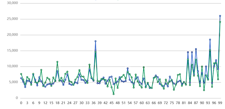
Figure 1. Fitting effect.

Where green represents predicted values, and blue represents actual values. The predicted house rent curve generated by this model demonstrates good predictive performance, closely following the actual trend of house price changes (Figure 1).

4. Conclusion

In conclusion, this study analyzed the rental prices of 400 houses in various districts of Shanghai. Six variables potentially influencing house rent were proposed, and multiple linear regression analysis was conducted. The analysis presented in this paper is effective and accurate because Pearson correlation coefficient tests were performed on all variables before using the multiple linear regression model.

The multiple linear regression model aimed to identify variables strongly related to house rent. To more accurately and rigorously identify these variables, related terms were incorporated, and further analysis was conducted using stepwise regression models. Ultimately, variables representing the number of rooms and whether there is a nearby subway station were excluded, while variables representing house size and renovation level were retained, with house size being the primary factor influencing house rent.

Through this research, individuals seeking to rent houses can have a rough reference and make informed decisions on where to rent. However, many factors were not considered, or variables with weaker correlations, such as house orientation and floor level. People can refer to more suggestions when deciding to rent, ultimately making a more informed decision.

References

[1]. Wang S, Wang Y and Shen Y 2023 The Impact of Supportive Housing Policy Scenarios on Marriage and Fertility Intentions: A Vignette Survey Experimental Study in Shanghai, China. Popul Res Policy Rev, 42, 96.
[2]. Akakuru O C, et al. 2023 Application of artificial neural network and multi-linear regression techniques in groundwater quality and health risk assessment around Egbema, Southeastern Nigeria. Environ Earth Sci, 82, 77.
[3]. Khandaskar S, Panjwani C, Patil D and Bajaj P 2023 House and Rent Price Prediction System using Regression. 2023 International Conference on Sustainable Computing and Smart Systems (ICSCSS), Coimbatore, India, 1733-1739.
[4]. Wen Y D, Wu Y Y and Li H 2024 Institutions, urban space, and residential markets in globalizing Shanghai: A comparative study of housing sale and rental prices, Journal of Urban Affairs.
[5]. Dang G Y and Yang T 2014 Multiple Linear Regression Analysis of Influencing Factors of House Prices in Tangshan City. Journal of Hebei United University (Social Science Edition), 21-25.
[6]. Dai L and Li X T 2019 Analysis of Influencing Factors of Second-hand Housing Prices Based on Multiple Linear Regression Model: Taking a District in Chengdu as an Example. Henan Building Materials, 80-82.
[7]. Zhang Y 2023 Research on the Impact of the Rent in Shanghai Based on Multiple Linear Regression Model. Highlights in Science, Engineering and Technology, 38, 364-369.
[8]. Dai X, Bai X and Xu M 2016 The influence of Beijing rail transfer stations on surrounding housing prices. Habitat International, 55, 79-88.
[9]. Wang N, Wu W and Hu X Y, et al. 2018 The Heterogeneity of the Impact of Major Transportation Facilities on Residential Prices under Urban Crossing Rivers: A Case Study of Binjiang New City in Nanchang City. Urban Studies, 10, 123-130.
[10]. Wang J F 2013 Prediction Model of Commodity Housing Price Based on Multiple Linear Regression. Science and Technology Vision, 210.
Cite this article
Qin,Z. (2024). Research on the influencing factors of housing rental prices-take Shanghai housing rents as an example. Theoretical and Natural Science,38,160-165.
Data availability
The datasets used and/or analyzed during the current study will be available from the authors upon reasonable request.
Disclaimer/Publisher's Note
The statements, opinions and data contained in all publications are solely those of the individual author(s) and contributor(s) and not of EWA Publishing and/or the editor(s). EWA Publishing and/or the editor(s) disclaim responsibility for any injury to people or property resulting from any ideas, methods, instructions or products referred to in the content.
About volume
Volume title: Proceedings of the 2nd International Conference on Mathematical Physics and Computational Simulation
© 2024 by the author(s). Licensee EWA Publishing, Oxford, UK. This article is an open access article distributed under the terms and
conditions of the Creative Commons Attribution (CC BY) license. Authors who
publish this series agree to the following terms:
1. Authors retain copyright and grant the series right of first publication with the work simultaneously licensed under a Creative Commons
Attribution License that allows others to share the work with an acknowledgment of the work's authorship and initial publication in this
series.
2. Authors are able to enter into separate, additional contractual arrangements for the non-exclusive distribution of the series's published
version of the work (e.g., post it to an institutional repository or publish it in a book), with an acknowledgment of its initial
publication in this series.
3. Authors are permitted and encouraged to post their work online (e.g., in institutional repositories or on their website) prior to and
during the submission process, as it can lead to productive exchanges, as well as earlier and greater citation of published work (See
Open access policy for details).