1. Introduction

The Autoregressive Moving Average model with eXogenous inputs (ARMAX) has its theoretical foundation in the seminal AutoRegressive Moving Average (ARMA) model, which was originally introduced in the highly influential book “Time Series Analysis: Forecasting and Control” by Box and Jenkins in 1970 [1]. As a pivotal tool for investigating temporal data, the ARMA model comprises two key components: the AutoRegressive (AR) part and the Moving Average (MA) part.

The AutoRegressive (AR) component delineates the dynamic interdependence between a time series’ current realization and its own lagged values. The AR process of order p postulates that the present observation can be expressed as a linear aggregation of the p immediately preceding periods’ terms [2]. This encapsulates the inherent inertia or short-term memory within the temporal sequence. By fitting a polynomial function to historical data, the AR mechanism models the endogenous propagation pattern to forecast forthcoming values.

In a complementary fashion, the Moving Average (MA) component represents the influence of stochastic shocks and random disturbances on the current observation. The MA parameters of order q quantify the lingering impacts of white noise error terms originating in the previous q periods [3]. Thereby, the MA process characterizes the finite memory length for exogenous perturbations imposed on the series and to smooth transient fluctuations.

Specifically, the AR portion delineates the interrelationship between the current observation and its own historical values, while the MA portion delineates the accumulation of errors in the AR forecasts.

Built upon the ARMA model, the ARMAX model incorporates exogenous variables, allowing it to account for the influence of external factors. The inclusion of exogenous inputs enhances the versatility and predictive accuracy of the model for many real-world applications [4]. Since its inception, the ARMAX framework has become widely utilized in myriad disciplines including finance [5], econometrics [6], and engineering [7] for its effectiveness in multivariate time series modeling and forecasting.

In the practical implementation of ARMAX, the stability of polynomial coefficients corresponding to model parameters warrants detailed analysis. As demonstrated theoretically and empirically by the study [8], the overall stability of ARMAX systems hinges entirely on the stability of the AutoRegressive (AR) and Moving Average (MA) components, which is contingent on the distribution of their polynomial roots. Therefore, this work necessitates verifying the stability of parameter polynomial coefficients and incorporating stability criteria as constraints during ARMAX model optimization. By ensuring stable AR and MA polynomials through coefficient constraints, the implemented ARMAX structure can exhibit robust forecasting performance.

Stability verification for ARMAX model involves analyzing the parametric polynomial coefficients that characterize the model’s dynamics. Two primary methods exist - the Hurwitz criterion using matrix algebra, and the Schur-Cohn criterion based on polynomial transformations. This work implements the Schur-Cohn test to check ARMAX stability, with preliminary experiments also done to explore the Jury test criterion.

The Schur-Cohn criterion relies on applying the Schur transform to the polynomial expressed as a linear combination of itself and its reciprocal. This special transformation converts the original complex polynomial into a reduced single-variable polynomial of degree one, with an associated complex parameter \( γ \) . The magnitude of \( γ \) relative to the unit circle threshold indicates whether the roots of the original polynomial lie inside or outside the unit disk [9]. By recursively applying the Schur transform to \( γ \) , a complete set of stability parameter { \( {γ_{k}} \) } can be derived. According to the criterion, the necessary and sufficient condition for stability is that all \( {γ_{k}}≥0 \) . In effect, the Schur transforms map the polynomial to the complex plane, allowing root locations to be inferred from the \( {γ_{k}} \) parameters. Compared to directly solving the characteristic equation, this elegant approach enables efficient and robust stability characterization for ARMAX models of any order. The mappings avoid expensive root computations, while providing generalization beyond the limitations of Hurwitz or Jury criteria.

Comparatively, the Jury criterion studies the sign patterns of polynomial derivatives on the boundary, thereby inferring root locations indirectly.

After obtaining the stability parameter \( γ \) , this project uses the Automatic Differentiation method to process the parameter sequence, and ultimately achieves the control of model stability by limiting the threshold value of the stability parameter \( γ \) . The article [10] describes the basic ideas and applications of automatic differentiation. It states that automatic differentiation methods are used not just to compute derivatives of functions, but to derive rules for summing, differencing, product, and quotient differentiation of functions. Once these rules have been established, the process of differentiation is analogous to the process of finding the value of a function.In general statement, this automatic differentiation method is an implicit computational law which is based on arithmetic operations on ordered pairs to compute function values and their derivatives. This method is easy to program on a computer. The auto-differential method can obtain function values and derivative values directly from function definitions without explicitly deriving derivative formulas and avoids approximation errors in numerical differentiation.

In addition, the article lists extensions to automatic differentiation, including higher-order derivatives, multiple independent variables, etc., which can be combined with other forms of operations, such as interval operations, to provide information about functions and their derivatives over a range of variables.

The purpose of using the automatic differentiation function in this project is that after obtaining the \( γ \) parameters and their automatic differentiation, they can be added as constraints to an existing ARMAX model. The NLopt library needs to be applied at this stage.

NLopt (Nonlinear Optimisation) is an open source library designed to solve a wide range of nonlinear optimisation problems. As can be seen from the official documentation page, the NLopt library provides optimisation algorithms and interfaces for a wide range of optimisation and constraint limitation problems. Specifically, the NLopt library supports a wide range of mainstream programming languages including C, C++, Python, etc., providing developers with a wide choice of optimisation algorithms. This project uses a C++ interface to the NLopt library called NLopt C-plus-plus Reference, which provides developers with a way to call optimisation algorithms from the NLopt library from within a C++ program to help solve complex problems involving non-linear optimisation.

Finally, the test sets and datasets used in this project were generated by dynamic modelling, a methodology described in the paper [11], which proposes a new approach that uses implicit models to represent the parameters of the objective function to be optimised in predictive control. This means that it is no longer necessary to explicitly model the dynamics of the system but to directly parametrically model the control objective. This approach avoids the use of predictive models by optimising directly in parameter space. As the control process proceeds, the optimisation algorithm can adjust the parameters in real-time to accommodate changing system characteristics and control requirements. By using an implicit model, complex predictive models can be avoided, thus reducing the amount of model-building effort. Secondly, this approach reduces computational complexity because the optimisation process is performed directly in the parameter space, avoiding the computation of predictive models. Most importantly, this approach can provide better performance and faster convergence in some cases.

In summary, the overall objectives and process structure of the project are as follows:

• Definition of ARMAX Model: Begin by formulating the ARMAX model, explicitly defining the polynomial parameters for both the autoregressive lag term (AR) and the moving average lag term (MA). This initial ARMAX model serves as the foundation for subsequent steps.

• Application of Schur Transform for Parameter Sequence: Implement the Schur Transform technique to process the AR and MA polynomial parameters. This process yields a sequence of parameters, wherein each value is indicative of the model’s stability characteristics.

• Automatic Differentiation of Parameter Sequences: Employ automatic differentiation to compute the gradients of the obtained parameter sequence. These gradients hold pivotal significance as they are used to establish constraints in forthcoming optimization procedures.

• Incorporation of Constraints: Harnessing the capabilities of the NLopt library’s algorithms, introduce the γ-values and their corresponding gradients as constraints into the original ARMAX model. This step ensures that the resultant optimized model exhibits enhanced stability.

• Model Execution: Execute the modified ARMAX model using both the test dataset and the complete dataset. This step involves the optimization process aimed at elevating the model’s stability.

• Attainment of Optimization Results: Conclude the project by obtaining the optimized model parameters. Undertake a comparison of the Mean Square Error (MSE) metrics prior to and post-optimization, thereby gauging the efficacy of the optimization process.

This project was carried out in parallel with two other projects that used genetic algorithms to find parameter values for the ARMAX model (the work of X. Zhang) and the use of ACF to impose constraints on the ARMAX model (the work of G. Liu). The ultimate goal is to run the stability constraints in conjunction with the other two components to obtain the best model optimisation results

2. Methodology

2.1. Description of the ARMAX model structure

The core structure and process of this project is shown by Figure 1, which is summarised as the parameter selection process of the ARMAX model using the Schur transform and the automatic derivation technique, introducing the stability requirement into the constraints and using the optimisation algorithm to obtain the ARMAX model that takes into account both accuracy and stability.

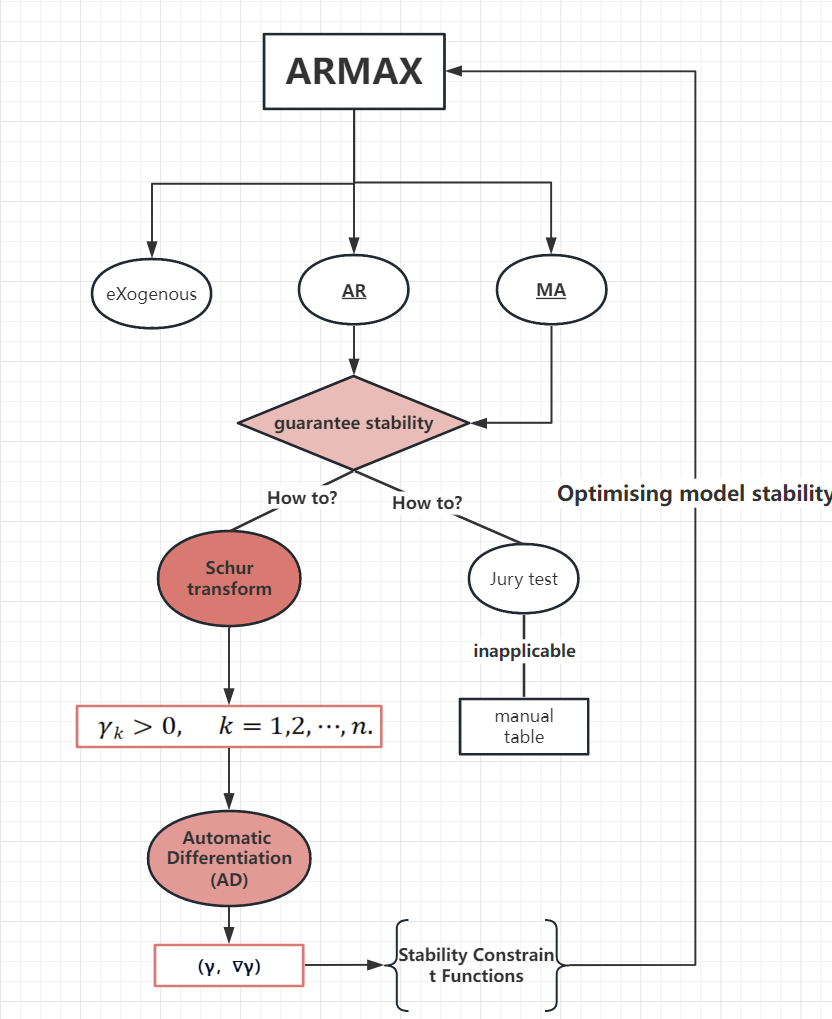
Figure 1. Core Project Structure and Process.

An ARMAX model can usually be represented as (1):

\( {Y_{t}}={ε_{t}}+\overset{\underset{p}{i=1}}{∑}{φ_{i}}{Y_{t-i}}+\overset{\underset{q}{i=1}}{∑}{θ_{i}}{ε_{t-i}}+\overset{\underset{r}{i=1}}{∑}{η_{i}}{X_{t-i}} \ \ \ (1) \)

where:

• \( {Y_{t}} \) - The value of the explanatory variable at moment t

• \( {ε_{t}} \) - Stochastic disturbance term

• \( {φ_{i}} \) - Autoregressive coefficient,i denotes the lag order

• \( {Y_{t-i}} \) - The value of the explanatory variable in the past i period

• \( {θ_{i}} \) - Moving average coefficient, i denotes lagged order

• \( {ε_{t-i}} \) - Random disturbance term for the past i periods

• \( {η_{i}} \) - Parameters of exogenous variables, i denotes lagged order

• \( {X_{t-i}} \) - Exogenous variable values in the past i period

p,q,r are the number of AR, MA and exogenous inputs, respectively. The AR term ( \( \sum _{i=1}^{p}{φ_{i}}{Y_{t-i}} \) ) describes the effect of past values on current values.The MA term ( \( \sum _{i=1}^{q}{θ_{i}}{ε_{t-i}} \) ) describes the effect of past perturbations and the exogenous variable term ( \( \sum _{i=1}^{r}{η_{i}}{X_{t-i}} \) ) describes the effect of external factors. This project is concerned with the stability of the AR and MA terms.

Taking the AR term as an example, expanding the AR part of (1) yields the following representation (2):

\( y(z):={a_{0}}+{a_{1}}{z^{-1}}+{a_{2}}{z^{-2}}+⋯+{a_{n}}{z^{-n}} \ \ \ (2) \)

Where:

• \( y(z) \) - Current time entry

• \( {a_{i}} \) - Parameters for the past i moments

• \( {z^{-i}} \) - Past ith time scale

• n \( ≥ \) 0 is mandatory

The AR part can be simply viewed as an n-dimensional discrete time series polynomial, to which the Schur transform and the Jury test are applied to discuss its stability respectively.

Discrete system stability is equivalent to the fact that all poles fall within the unit circle [12]. This condition is tantamount to the fact that the poles of the system are within the unit circle of the complex conjugate plane (Z-plane), which according to the Laplace transform, maps to the region of the negative semiaxis of the complex frequency plane (S-plane), as illustrated by Figure 2:

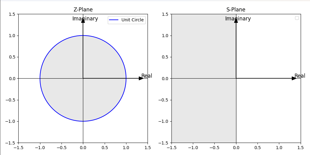
Figure 2. Mapping relations from the interior of the unit circle in the Z-plane to the negative semi-axis of the S-plane.

The Schur transform is first used to determine whether the roots of the polynomial are inside the unit circle. For an n-dimensional polynomial p of the form (3), we define its reciprocal polynomial \( {p^{*}} \) via (4):

\( p(z):={a_{n}}{z^{n}}+{a_{n-1}}{z^{n-1}}+⋯+{a_{0}} \ \ \ (3) \)

\( {p^{*}}(z):=\bar{{a_{0}}}{z^{n}}+\bar{{a_{1}}}{z^{n-1}}+⋯+\bar{{a_{n}}} \ \ \ (4) \)

If p is a polynomial of degree n ≥ 1 given by (3), the polynomial Tp of degree n-1 defined by (5) is called the Schur transform of p.

\( Tp(z):=\overline{{a_{0}}}p(z)-{a_{n}}{p^{*}}(z) \)

\( =\sum _{k=0}^{n-1}(\overline{{a_{0}}}{a_{k}}-{a_{n}}\overline{{a_{n-k}}}){z^{k}} \ \ \ (5) \)

The Schur transform of a polynomial with a degree of 0 results in the zero polynomial. It’s important to highlight that the Schur transform of a polynomial p is influenced by the degree assigned to p itself, rather than solely being determined by the function p.

Then we need to define the iterated Schur transform \( {T^{2}}p \) , \( {T^{3}}p \) , ... , \( {T^{n}}p \) by (6), where \( {T^{k-1}}p \) should be treated as a polynomial of order n-k+1 even if the leading coefficient is zero.

\( {T^{k}}p:=T({T^{k-1}}p), k=2,3,⋯,n. \) (6)

At the same time, we can note that Tp(0), of the form (7), will always be a real number.

\( Tp(0)=\overline{{a_{0}}}{a_{0}}-{a_{n}}\overline{{a_{n}}}={|{a_{0}}|^{2}}-{|{a_{n}}|^{2}} \) (7)

Here we set scale parameters (8):

\( {γ_{k}}:={T^{k}}p(0) \) (8)

We can obtain a theorem that all poles of the n-dimensional polynomial p are outside the unit circle if and only if (9) holds.

\( {γ_{k}} \gt 0, k=1,2,⋯,n. \) (9)

The calculation of \( {γ_{k}} \) is called the Schur-Cohn algorithm [9]. The algorithm is characterised by converting the polynomials into Schur parameter form and recursively performing Schur transformations. Each transformation produces a complex parameter \( γ \) . If all the resulting real parts of \( γ \) are non-negative, all the roots of the initial polynomial are outside the unit circle. On the contrary, if there exists one \( γ \) parameter whose real part is negative, then at least one root of the polynomial is inside the unit circle.

The most important feature of the algorithm is that it is computed using the coefficients of each term of the polynomial and the complex characteristic equations can be avoided. The method is low arithmetic and applicable to any high-order polynomials.

Recalling (2) and (3), we want (2) to be stable, we need to transform it into the form of (3), which corresponds to poles outside the unit circle, i.e., \( {γ_{k}} \gt 0 \) . At this point, the poles of (2) are inside the unit circle, which yields the stability conclusion.

Since the polynomial coefficients of the AR and MA parts of our current application are real numbers, the Schur transform can be simplified to (10):

\( Tp(z):={a_{0}}p(z)-{a_{n}}{p^{*}}(z) \)

\( =\overset{\underset{n-1}{k=0}}{∑}(\cdot {a_{0}}{a_{k}}-{a_{n}}{a_{n-k}}){z^{k}} \) (10)

We create a new project, using the C++ programming language, complete the programming of the Schur transform and test it with two sets of sequences of known stability, as shown in appendix for details.

Since the input to the Schur transform is practically related to the polynomial coefficients only, we create a vector P, store the coefficients of each term of the original polynomial in order, and then process vector P with the reverse function to obtain the inverted sequence invP. We then create the function entitled SchurTransform, which has two inputs, the first being the vector P constant and the second being the reference vector variable P_red. Calculate the data according to (10), and return the result to the reference vector variable P_red using the push_back function, at which time P_red^[0] is the \( γ \) value under the dimension, and the obtained P_red is the new sequence after the dimension is reduced by 1. Then create a for loop in the main function with the number of polynomial coefficients, and use SchurTransform function inside the loop. Assign the obtained P_red to P to implement the computation of \( {T^{k}}p \) and obtain \( {γ_{k}} \) .

Take the example of a set of time series (11):

\( p(z)={z^{3}}-1.3{z^{2}}-0.08z+0.24 \) (11)

The sequence is known to be stable and the process of performing the Schur transformation on it is shown in the Table 1 below:

Table 1. Example of applying schur transformrties to a polynomial

\( P \) is the input vector and \( invP \) is the inverse vector of P. The subscripts of both indicate the number of times they have gone through the Schur transform, and the number with the shaded background represents the \( γ \) -value; notice that only one element in \( {P_{3}} \) . The resulting \( {P_{4}} \) is null, but at this point it is possible to compute a \( γ \) -value, i.e., it is the \( {P_{3}} \) element itself.

2.2. Comparison of Jury test and Schur-Cohn algorithm

In this session, we also tried the Jury test criterion. Jury test is based on the discriminant theorem, which assesses the stability of a system by constructing a specific discriminant. The core idea of the method is to take the coefficients of the characteristic equations of the system as inputs and determine whether the system is stable or not by calculating the value of the discriminant.

After comparison, we found that the Jury test has limitations compared to the Schur transform:

Firstly, the Jury test can only determine whether a discrete sequence is stable or not in terms of its conclusions, and cannot provide the results of the calculations for each step. This makes it difficult to understand the details and influences of the discrete system stability problem [13]. For example, in a complex discrete system, if the Jury test concludes that the system is unstable, we cannot intuitively understand which coefficients or factors contributed to this result. This opacity limits our understanding of the system stability problem.

In contrast, the Schur transform provides more visualisation and tractability in determining the stability of discrete systems. By transforming the coefficients of a discrete system into \( γ \) values, we can visualise the impact of each dimension. This helps us to better understand the stability characteristics of the system and how to achieve stability by adjusting the parameters.

The Jury test can become complex and cumbersome when dealing with higher-order discrete systems. As the order of the system increases, the tables and calculations of the Jury test will increase dramatically, resulting in computation and judgement becoming difficult. Schur transform is relatively more suitable for higher order systems because it has better scalability by handling the coefficients through the multiplication and inverse of matrices. It can handle the stability judgement of higher-order systems more efficiently and also provide an intuitive presentation of the results. A comparison of the time complexity of the two is shown in the Figure 3 below:

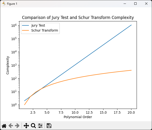
Figure 3. Comparing the time complexity of Jury test and Schur transform algorithms.

It can be appreciated that the time complexity of the Jury test increases linearly, while the time complexity of the Schur transform is logarithmic. For polynomials with coefficients more than 4 terms, it is more appropriate to use Schur transform, which explains the fact that Jury test is more suitable for manual handwritten forms.

2.3. Application steps of Schur-Cohn algorithm

After successfully implementing the Schur transform function, we apply it to the ARMAX model. We branch the original ARMAX model code and rename it to “CarmaxModel3.h” and “CarmaxModel3.cpp”. In the structure of the header file, we create functions named “calcAutoregressiveGammaValues” and “calcMovingAverageGammaValues”, and coding the two functions in the source file, as shown in appendix for details.

For calcAutoregressiveGammaValues Function, it calculates the \( γ \) values for the autoregressive polynomial. It iterates through the AR coefficient vector “arCoefficients” and applies the Schur transform using the SchurTransform function. The resulting \( γ \) values are pushed into “gamma_autoregressive” vector.

Similarly, another function iterates through the MA coefficient vector “maCoefficients” and applies the Schur Transform using the same SchurTransform function. The calculated \( γ \) values are stored in the “gamma_movingAverage” vector.

Both functions follow a similar pattern of applying the Schur Transform iteratively to the coefficient vectors, which eventually produces the \( γ \) values for each polynomial order.

After implementing the \( γ \) values for the polynomial coefficients, we need to extend the Schur transform code with a reference to the existing Dual Numbers file to include automatic differentiation to obtain the gradient, which is applied to the subsequent stability constraints.

Finally we proceeded to add constraints to the AR and MA components. When calling the polynomial coefficients of each part,first specify the data structure of the ARMAX model as shown in Figure 4:

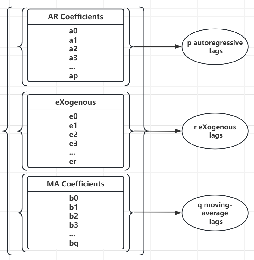
Figure 4. Data structure of polynomial coefficients.

It can be seen that the coefficients of the three parts are stored in the same data structure at the same time, so lags needs to be clarified when calling to initialise the other parts.

The “arCoefficientFn” function is defined first. This function is used to compute the constraints on the coefficients of an autoregressive polynomial for use in optimisation or constraint solving algorithms. This function takes several arguments: noConstraints (the number of constraints to compute), constraintVector (an array storing the values of the computed constraints), noParameters (the number of parameters to optimise), parameters (an array containing the current parameter values), grad (an array storing the values of the gradient) and data (pointer to additional data).

This function computes the constraints on the coefficients of the autoregressive polynomial using the Schur transform method (implemented by the SchurTransform_DualNumber function) and Dual Numbers for automatic differentiation.

It first extracts the autoregressive lags from the provided model instance “pArmaxModel”. The AR parameter values are copied into vectors of “dualNumber_t” objects, each initialised with the parameter values and indexes.

Each parameter is then iterated over, the Schur transform is computed using logarithms, and the result is stored in the “gamma_autoregressive” vector.

The computed \( γ \) is copied into the constraint vector. The grad array is also provided, and the gradient value is computed using the gradient value of the pair of even numbers and stored in the appropriate location in the grad array.

The process of defining the “maCoefficientFn” function is similar to the above, and since the coefficients of the MA part are at the end of the sequence, the offset is added to ensure that the data is read correctly.

Finally, we use the NLopt library to add the Schur stability coefficients as constraints in the optimisation process. Specifically use the nlopt_add_inequality_mconstraint function: this function comes from the NLopt optimisation library.

It is used to add inequality constraints to the optimisation problem. It takes several arguments: opt: optimisation object or instance. The number of constraints to add (e.g. m_arCoefficients.size() for autoregressive constraints and m_maCoefficients.size() for moving average constraints).

In this procedure it is necessary to call the previously constructed constraint functions, i.e. arCoefficientFn for autoregressive constraints and maCoefficientFn for moving average constraints.

The code adds constraints to the optimisation problem based on the Schur stability coefficients of the ARMAX model, as shown in appendix for detail.

The intent is that by adding these constraints, the optimisation process ensures that the resulting ARMAX model meets the stability criteria implied by the Schur stability coefficients. The code integrates the Schur stability constraints into the optimisation process, allowing the autoregressive and moving average coefficients of the model to be adjusted while maintaining stability.

After debugging, writing and compiling the code, we use the test set and the dataset to train the model with the added stability constraints. The basic idea is to iterate the model by setting the number of ARs, eXs and MAs from 1 to 10 and 0 to 9, and continuously monitor and record the output MSE and the corresponding \( γ \) values of the AR and MA parts of the model for each run to obtain the results of the project.

3. Results & Evaluation

We trained the ARMAX model using both test and training sets and integrated the newly incorporated stability constraints. The basic approach is to iteratively train the model by systematically varying the number of AR and exogenous inputs from 1 to 10, and the number of MAs from 0-9, using the three sets of parameters as inputs. The entire number of iterations is 1000, and during this iteration process, we continuously track and record the mean square error (MSE) output generated by the model to obtain the results of the training. In addition, we simultaneously recorded the corresponding \( γ \) values associated with the AR and MA components of the model. These \( γ \) values reflect the nature of the stability characteristics of the ARMAX framework. The initial data obtained are shown in Table 2 below:

Table 2. Partial data results with AR factor of 1.

Due to the length of the data being excessive (1000 rows), only some of the results are shown here. We migrated the data results to a table and used the table tool to arrange and sort the analyses.

Sorting the test MSE values in ascending order, we get the following well-performing portion of the data, as shown in Table 3:

Table 3. The partial experimental data featured minimum test MSEs.

Note that this portion of the data includes numerous MA (Moving Average) terms with a value of 0. When the count of MA terms is 0, the entire model becomes simplified, leading to a reduction in computational load. Consequently, the resulting Mean Squared Error (MSE) tends to be lower. The utilization of this parameter subset can indeed showcase the performance of the simplified model. However, its significance in terms of the comprehensive stability analysis of the complete ARMAX model is limited.

Use the table tool to filter out the parts with MA equal to 0 and re-sort them in ascending order according to test MSE, and the results obtained are shown in Table 4:

Table 4. The partial experimental data without 0 MA terms.

We find the results of model runs without stability constraints for the same parameter case and plot them in Table 5 below:

Table 5. Comparison of model test mse data before and after adding stability constraints

(p,q,r) are the number of AR terms, the number of MA terms and the number of external input terms respectively.

Data with this property are 168 out of 1000 sets of parameters.

We compare the non-stable MSE data produced after using the genetic algorithm (this part of the data comes from the work of X. Zhang) with the MSE data after applying the stability constraints and get the Table 6 below:

Table 6. Comparison of model test mse data after using the genetic algorithm and after adding stability constraints

(p,q,r) are the number of AR terms, the number of MA terms and the number of external input terms respectively.

These exceptions occurred 28 times in 100 iterations of GA.

We then compare the non-stable MSE data produced after apply the ACF constraints (this part of the data comes from the work of G. Liu) with the MSE data after applying the stability constraints and get the Table 7 below:

Table 7. Comparison of model test mse data after using the acf constraints and after adding stability constraints

(p,q,r) are the number of AR terms, the number of MA terms and the number of external input terms respectively.

We then demonstrate the other extreme case. Sorting the Test MSEs in descending order yields the results shown in Table 8 below:

Table 8. Results characterised by large test MSE data

It can be observed in many combinations of parameters. After stability restriction, the obtained values of train MSE are often Inf or 2.25823 and the value of test MSE is 1.96825.

Finally, we extracted some outliers. There were 22 outliers out of 1000 experimental results.

4. Discussions

A primary observation that can be made is the evident enforcement of stability restrictions during the model’s execution. This is evident when we examine the sequence of \( γ \) values associated with the AR and MA components. Upon closer inspection, it becomes apparent that all the \( γ \) values are either greater than or very close to 0. Even in cases where values are slightly below 0, such as -6.71342e-12, they can be interpreted as negligible systematic errors within the realm of auto-differencing tolerance.

A comparative analysis of the aforementioned sections underscores the substantial impact of stability constraints on the outcomes. In cases where the model parameters were initially deemed unstable, such as the configuration (4, 1, 10), the introduction of stability restrictions led to a remarkable reduction in Test MSE. Specifically, the Test MSE, which was initially at an excessively high and problematic level, was successfully brought down to a range considered normal. This transformation rendered the previously challenging parameter configuration, (4, 1, 10), viable and practically applicable.

Certain parameter combinations that initially exhibited an unstable tendency also demonstrate noticeable improvements when stability restrictions are applied. For instance, consider the parameter set (7, 1, 9), which originally yielded a high MSE value of 21.238, indicative of instability. However, following the imposition of stability restrictions, the MSE value drastically drops to 0.10, signifying a remarkable enhancement in usability.

This pattern suggests that similar parameter combinations could experience enhanced usability by incorporating stability restrictions. On the contrary, parameter sets that were inherently stable, such as (4, 1, 1), consistently maintain nearly identical MSE values before and after the application of stability restrictions. This finding indicates that stability restrictions do not significantly interfere with the performance of initially stable parameter combinations.

The occurrence of Inf values in the training MSE, along with a test MSE value of 1.95825, suggests that there might be issues related to convergence during the training process. The presence of Inf values could indicate that the optimization algorithm struggled to find optimal parameter values, leading to such results. Interestingly, both the \( γ \) values for the AR and MA components are observed to be 0, indicating that stability constraints are enforced on the coefficients of both the AR and MA polynomials.

In the context of the optimization algorithm’s logic, it calculates the current \( γ \) value and adjusts the coefficients through automatic differentiation if they are deemed unstable. However, due to the mandatory stability requirement, the exact nature of the modified coefficients remains uncertain. This situation could arise from the imposition of stability constraints, causing the polynomial coefficients to converge to an adjustable limit value where further changes are restricted. Consequently, the model might not fully perform its predictive function, resulting in consistent outcomes across various parameter sets.

In light of these results, it becomes evident that the ARMAX model, under this scenario, ensures stability. However, this stability assurance might come at a cost. While the model maintains stability, its predictive functionality could be compromised due to the limited adjustments allowed by the stability-enforced coefficient convergence. This trade-off between stability and predictive performance should be carefully considered when interpreting the results of the ARMAX model under these conditions.

Finally, we purposefully analysed these 22 sets of outlier data and observed some common features. These data generally exhibit a small mean square error (MSE) on the training set and a large MSE on the test set. This may indicate that the model performs well on the training data but poorly on the unseen data, which is consistent with an overfitting problem.

The root cause of overfitting is that the model overfitted the noise and specific samples in the training data during training, thus failing to generalise well to new data. In these 22 data sets, we noticed a common feature of the AR part, namely, unusually small \( γ \) values, which implies that the stability constraints are not well enforced under these parameter combinations. For example, the \( γ \) value in parameter combination (8, 1, 10) is -12.3496, which is very rare in the whole training results. This may be due to individual anomalies in the AR part of the training process and is not generalisable or reproducible. In order to determine the root cause of the problem, it is necessary to train the model several times and compare the results.

Furthermore, in combination with the occasional Inf phenomenon, we can speculate that stability limitations may have contributed to the problem of long computation times. Therefore, subsequent work needs to further optimise the algorithm to reduce the computational complexity in order to handle the stability constraints more efficiently while improving the training efficiency of the model.

5. Conclusions

In this project, we follow a process structure that firstly implements the Schur transform based on the properties of the AR and MA parts of the model, and further implements its autonmetic differentiation function, and finally as a stability constraints algorithm to achieve the optimisation of the existing ARMAX model. The model is then trained using a test set and a dataset, focusing on the performance and impact of the ARMAX model with the introduction of stability constraints. Through a series of experiments and analyses, a number of important conclusions and findings are drawn, providing insights into the stability and performance enhancement of the model.

Based on the data obtained after training, it is shown that in many cases, the performance of the model is significantly improved by introducing stability constraints. In particular, for the originally unstable parameter combinations, after adding stability constraints, the MSE of the model is reduced from abnormally high values to normal levels, which proves the effectiveness of the stability constraints.

We also note that the stability constraint may cause some computational problems, such as the appearance of Inf values. This may be due to the fact that the stability constraint increases the complexity of model training, and further optimisation of the algorithm is required to cope with these problems.

As for the data performance with smaller MSE on the training set and larger MSE on the test set for certain parameter combinations, this may be due to an overfitting problem, i.e., the model performs well on the training data but poorly on the test data. For this part of the data, we need to take more measures to prevent the model from overlearning the training data in order to improve its generalisation ability.

In addition, we cited the outlier data, such as cases where stability constraints did not effectively constrain certain parameter combinations. For these problems, we need to conduct more in-depth research and experiments on the specific changes in the polynomial coefficients within the model in order to identify the root causes and propose solutions.

The research in this project has empirically studied and deeply analysed the stability constraints of the ARMAX model, and the performance of the model after stability constraints has been improved by about 10% ((number of parameter combinations that effectively improve the performance - anomalous combinations)/total number of trials). Our work not only from implementing and verifying the validity of the stability constraints, but also reveals the possible causes of model overfitting problems and anomalies.

However, there are still many issues that need to be further investigated, including more extensive parameter combination experiments, more rigorous stability analyses and more optimal algorithm designs.

6. Future Work

This project was only an initial attempt to investigate the stability constraints of the ARMAX model and there is still much work to be done in the future:

• Using multiple datasets: Due to the time requirement of the project, only one dynamic dataset was used this time. In the future, we can train the ARMAX model with multiple datasets and compare and analyse the results obtained to obtain more accurate results.

• Explore more stability measurements: Although this study uses the Schur transformation with \( γ \) values as an indicator of stability, exploring other stability measures could provide a more complete picture of the model’s behaviour. Investigate methods that consider system matrix eigenvalues or other stability criteria.

• Optimising Algorithms: As noted in the study, a number of computational issues and occurrences of “Inf” values were noted. Future work will focus on optimising the underlying algorithms, possibly by exploring more efficient optimisation techniques or parallel processing to reduce training time and improve stability.

• Investigating individual polynomial coefficients: There is a need to develop research to explain the impact of individual coefficients on overall stability and performance. This will help provide insight into the trade-off between stability constraints and prediction accuracy.

By addressing these areas in future research, we can deepen our understanding of ARMAX model stability and performance and develop more robust and reliable modelling techniques for a variety of applications. These further studies will help to better understand and apply the ARMAX model for stability and performance optimisation in real-world problems.

In addition, in the future it will be necessary to merge the other two projects, which are the use of genetic algorithms to find the values of the ARMAX model parameters and the use of ACF to impose constraints on the ARMAX model. The ultimate goal is to run the stability constraints in conjunction with the other two components to obtain the best model optimisation results.

Acknowledgment

How time flies. I am honoured to end a wonderful year of my master’s degree with my final project. During this time, I have met friendly classmates and dedicated professors, and I have enjoyed this year very much.

First of all, I would like to express my sincere gratitude to my supervisor, who has guided and helped me in every step of the project. He went to great lengths to describe the structure and details of the project to me, and I probably could not have done it without his help!

Also, I would like to thank the other two students who worked on parallel projects, we shared the training results of our respective projects with each other. I am looking forward to the future ARMAX modelling results when our work is merged! As our supervisor said, our projects are all about throwing stones into the river and one day we will reach the other side!

I will miss everything that has happened here again and again in the time to come! Once again, I would like to express my sincere gratitude to all the professors and students who have helped me.

References

[1]. Khashei, M., & Bijari, M. (2021). A novel hybridization of artificial neural networks and ARIMA models for time series forecasting. Applied Soft Computing, 100,106983. https://doi.org/10.1016/j.asoc.2020.106983
[2]. J. D. Hamilton, Time series analysis. Princeton, N.J. ; Chichester: Princeton University Press, 1994.
[3]. Liu, B., Nowak, R. D., & Tsakiri, K. (2019). Automatic time series modeling with pruned ARMAX. IEEE Access, 7, 121365–121377. https://doi.org/10.1109/ACCESS.2019.2937966
[4]. W. Palma, Long-memory time series : theory and methods. Hoboken, N.J.: Wiley, 2007.
[5]. S. Khan and H. Alghulaiakh, “ARIMA model for accurate time series stocks forecasting,” International journal of advanced computer science & applications, vol. 11, no. 7, pp. 524–528, 2020, doi: 10.14569/IJACSA.2020.0110765.
[6]. Bouallègue, Z. B. (2020). Forecasting frameworks based on the hybridization of prominent data science techniques: Illustrations using international industrial production series. Expert Systems with Applications, 158, 113547. https://doi.org/10.1016/j.eswa.2020.113547
[7]. Raza, M. Q., & Khosravi, A. (2020). Towards better time series forecasting with incremental learning strategy. Information Sciences, 544, 413–427. https://doi.org/10.1016/ j.ins.2020.07.023
[8]. K. M. Hangos and I. T. Cameron, Process Modelling and Model Analysis. San Diego, CA: Academic Press, 2001.
[9]. P. Henrici, Applied and computational complex analysis. New York ; London (etc.): Wiley-Interscience, 1974.
[10]. Wei, L., & Guo, T. (2020). A pruned ARMAX model for short-term wind speed forecasting. Energy, 193, 116751. https://doi.org/10.1016/j.energy.2019.116751
[11]. J. A. Rossiter, B. Kouvaritakis, and L. Huaccho Huatuco, “The benefits of implicit modelling for predictive control,” in Proceedings of the 39th IEEE Conference on Decision and Control (Cat. No.00CH37187), 2000, vol. 1, pp. 183–188 vol.1. doi: 10.1109/CDC.2000.912755.
[12]. Chakraborty, T., & Michael, A. (2021). Application of ARMAX model with exogenous input for forecasting electricity price. Energy, 237, 121533. https://doi.org/10.1016/j.energy. 2021.121533
[13]. R. C. Dorf and R. H. Bishop, Modern control systems., 12th ed., International ed. / Richard C. Dorf, Robert H. Bishop. Boston, [Mass.] ; London: Pearson, 2011.
Cite this article
He,S. (2024). Training ARMAX model based on the Schur-Cohn algorithm to guarantee stability. Theoretical and Natural Science,38,213-228.
Data availability
The datasets used and/or analyzed during the current study will be available from the authors upon reasonable request.
Disclaimer/Publisher's Note
The statements, opinions and data contained in all publications are solely those of the individual author(s) and contributor(s) and not of EWA Publishing and/or the editor(s). EWA Publishing and/or the editor(s) disclaim responsibility for any injury to people or property resulting from any ideas, methods, instructions or products referred to in the content.
About volume
Volume title: Proceedings of the 2nd International Conference on Mathematical Physics and Computational Simulation
© 2024 by the author(s). Licensee EWA Publishing, Oxford, UK. This article is an open access article distributed under the terms and
conditions of the Creative Commons Attribution (CC BY) license. Authors who
publish this series agree to the following terms:
1. Authors retain copyright and grant the series right of first publication with the work simultaneously licensed under a Creative Commons
Attribution License that allows others to share the work with an acknowledgment of the work's authorship and initial publication in this
series.
2. Authors are able to enter into separate, additional contractual arrangements for the non-exclusive distribution of the series's published
version of the work (e.g., post it to an institutional repository or publish it in a book), with an acknowledgment of its initial
publication in this series.
3. Authors are permitted and encouraged to post their work online (e.g., in institutional repositories or on their website) prior to and
during the submission process, as it can lead to productive exchanges, as well as earlier and greater citation of published work (See
Open access policy for details).