1. Introduction

Black-Scholes model has gained much significance in the academic field of financial mathematics. Mathematical concepts have been used in the financial market since 1202 when Fibonacci started to calculate the present value of a cash-flow when he was trying to solve a number theory problem. According to Akyıldırım and Soner [1], Louis Bachelier first apply Brownian motion trajectories to simulate the fluctuation in stock price and to compute price of some options in 1900s before Norbert Wiener provides the rigorous proof. Kiyoshi Ito invented the famed Ito formula in 1951, which was one of the fundamentals of stochastic calculus and is still widely used in mathematical finance. After the breakthrough of Black-Scholes Formula in 1973, Mathematicians and financial engineers further investigated the features of special types of options based under Black-Scholes Market assumptions. It could be very hard to derive the analytic solution to options which depends on the path of the stock price. In these cases, using a numerical method is more efficient. In this article, we explore three approaches to pricing options: the martingale theory, related PDEs, and numerical simulations. We start from introducing the concept of continuous time Black-Scholes Model together with Monte-Carlo simulation. Then we go over the steps to derive pricing formula for several exotic options, including Chooser’s option, Barrier option, Look-back option and Asian option. For each one, we included the analytic solutions, juxtaposed by the corresponding Monte Carlo simulation and also change the value of some parameters to observe the consequences on option price. We will compare the Monte Carlo estimations to the corresponding analytic solutions. The Roger and Shi’s study was thoroughly examined in the Asian option part since we heavily rely on their findings because the embedded PDE is very difficult to solve or to find a numerical solution. As a consequence, we provide the comparison of several valid techniques.

1.1. Mathematical Background

Consider the probability space \( (Ω,F,P) \) . In this triple, \( Ω \) is the set of all possible outcomes of a underlying pricing. \( F={\lbrace {F_{t}}\rbrace _{t \lt =T}} \) is a collection of \( σ \) -field \( {F_{t}} \) can be interpreted as the “Information Stream”, given \( {F_{t}} \) means we are access to all the history before time \( t \) . \( P \) measures how an event (or many events) is likely to happens. Therefore, the cost of a derivative written on an underlying may be determined using the probability distribution of that underlying. The following is a reformulation of the results in Yan and Evans [2,3].

Theorem 1.1. (Ito Chain Rule)For stochastic process \( {X_{t}} \) s.t:

\( d{X_{t}}=μ(t,{X_{t}})dt+σ(t,{X_{t}})d{W_{t}} (1) \)

Where \( μ∈{L^{1}}(0,T) \) and \( σ∈{L^{2}}(0,T) \) . Let \( {Y_{t}}=f(t,{X_{t}}) \) , then:

\( d{Y_{t}}=(\frac{df}{dt}+\frac{df}{dx}μ+\frac{1}{2}\frac{{d^{2}}f}{d{x^{2}}}{σ^{2}})dt+σ\frac{df}{dx}dW (2) \)

Theorem 1.2. (Ito Product Rule) Suppose the system of SDEs is :

\( \begin{matrix} & d{X_{1}}={μ_{1}}dt+{σ_{1}}d{W_{t}} \\ & d{X_{2}}={μ_{2}}dt+{σ_{2}}d{W_{t}} \\ \end{matrix} (3) \)

over \( t∈ [0,T] \) , where \( {μ_{1}},{μ_{2}}∈{L^{1}}(0,T) \) and \( {σ_{1}},{σ_{2}}∈{L^{2}}(0,T) \) then :

\( d({X_{1}}{X_{2}})={X_{1}}d{X_{2}}+{X_{2}}d{X_{1}}+d{X_{1}}d{X_{2}} (4) \)

1.2. Continuous Time Model

In continuous time setting, it is assume that there only exists two financial instruments in the market, they are Stock \( S \) and saving account \( B \) . The stock price is stochastic and returns are risky, while saving in the bank is risk-free. It was also assumed that the stock pays no dividends, traders are free to make transactions, volatility \( σ \) is an invariable parameter in the short run and the stock price’s dynamic follows:

\( {S_{t}}={S_{0}}{e^{σ{W_{t}}+(μ-\frac{{σ^{2}}}{2})t}} (5) \)

where \( {W_{t}} \) denotes a Brownian motion and \( μ \) represents mean-return rate, which is included in Black and Scholes [4]. The stochastic differential equation (SDE) of stock can then be easily extracted using Ito’s formula. :

\( \begin{matrix}d{S_{t}}=df(t,{W_{t}}) & ={S_{t}}(μ-\frac{{σ^{2}}}{2}+\frac{{σ^{2}}}{2})dt+σ{S_{t}}d{W_{t}} \\ & =μ{S_{t}}dt+σ{S_{t}}d{W_{t}} \\ \end{matrix} (6) \)

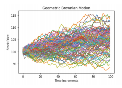
This SDE is known as the Geometric Brownian Motion. On the other hand, bank savings is continuously accelerated by a short-term constant interest rate. Hence this gives the SDE for risk-free asset :

\( d{B_{t}}=r{B_{t}}dt  and  {B_{t}}={e^{rt}} (7) \)

Let’s examine the discounted stock price procedure in more detail, i.e. \( {\lbrace \frac{{S_{t}}}{{B_{t}}}\rbrace _{\lbrace t∈T\rbrace }} \) . Let \( {F_{t}} \) be the smallest \( σ \) -field generated by random variable \( {W_{t}} \) . Similar to the discrete-time model, we would like to determine a risk-neutral measure which will enable us to swap out the mean-return rate with a fixed interest rate in the model. Such a measure is guaranteed to exist under the BS model assumption. Precisely, it is stated in the following theorem :

Theorem 1.3. A unique equivalent martingale measure(EMM) is obtainable when a market is complete and there is no chance for arbitrage. Completeness indicates that for any contingent claim, there is a portfolio replicating it. Arbitrage means making money without taking any risks. This theorem is known as the Fundamental theorem of option pricing.

For process \( S_{t}^{*}=\frac{{S_{t}}}{{B_{t}}} \) , the EMM \( Q \) is given by the Radon-Nikodym derivative :

\( \frac{dQ}{dP}=exp⁡(\frac{r-μ}{σ}{W_{T}}-\frac{1}{2}{(\frac{μ-r}{σ})^{2}}T),  for  t∈ [0,T] (8) \)

And \( S_{t}^{*}=\frac{{S_{t}}}{{B_{t}}} \) is a martingale under measure \( Q \) :

\( \begin{matrix}E[\frac{{S_{t}}}{{B_{t}}}\frac{dQ}{dP}∣{F_{u}}] & =E[\frac{{S_{u}}{e^{σ{W_{t-u}}+(μ-\frac{{σ^{2}}}{2})(t-u)}}}{{e^{ru}}{e^{r(t-u)}}}{e^{\frac{r-μ}{σ}{W_{t-u}}-\frac{1}{2}{(\frac{μ-r}{σ})^{2}}(t-u)}}∣{F_{u}}] \\ & =\frac{{S_{u}}}{{B_{u}}}{e^{(μ-r-\frac{{σ^{2}}}{2}-\frac{1}{2}{(\frac{μ-r}{σ})^{2}})(t-u)}}E[{e^{(σ+\frac{r-μ}{σ}){W_{t-u}}}}∣{F_{u}}] \\ & =\frac{{S_{u}}}{{B_{u}}}{e^{(μ-r-\frac{{σ^{2}}}{2}-\frac{1}{2}{(\frac{μ-r}{σ})^{2}})(t-u)}}{e^{\frac{1}{2}{(σ+\frac{r-μ}{σ})^{2}}(t-u)}} \\ & =\frac{{S_{u}}}{{B_{u}}}={E^{Q}}[\frac{{S_{t}}}{{B_{t}}}∣{F_{u}}] \\ \end{matrix} (9) \)

Moreover, it also satisfies the SDE:

\( dS_{t}^{*}=σS_{t}^{*}dW_{t}^{Q}, Where W_{t}^{Q}={W_{t}}+\frac{μ-r}{σ}  is a brownian motion under Q \)

Thus:

\( d{S_{t}}=r{S_{t}}dt+σ{S_{t}}dW_{t}^{Q} (10) \)

Intuitively, we are able to foresee the stock price in the future only given the price today. The rigorous proof of the above steps can be found in the books of Musiela and Rutkowski 7 and Bingham and Kiesel 2. For simplicity, we will write \( W_{t}^{Q} \) as \( {W_{t}} \) and use \( r \) instead of \( μ \) imagining we are already in a risk-neutral world.

Returning to the subject of option pricing, there are two different approach. The first technique involves creating a partial differential equation using a replicating portfolio and defining the boundary based on the properties of a certain option to solve the PDE. Another method is using probability theory to compute the expectation. We will start from the first one by defining Wealth process and hedging portfolio. The following definition is taken from Musiela and Rutkowski [5]:

Definition 1.1 (Wealth Process). The pair \( {ϕ_{t}}=({a_{t}},{b_{t}}) \) is the portfolio consisting of \( {a_{t}} \) and \( {b_{t}} \) . Here \( {a_{t}} \) represents the amount of shares holding at time \( t \) , while \( {b_{t}} \) represents number of money invested in risk-free asset at time \( t \) . Then the the value of portfolio \( ϕ \) at time \( t \) is \( {V_{t}}({ϕ_{t}})={a_{t}}{S_{t}}+{b_{t}}{B_{t}} \) . In consequence, the strategy relies on time and stock price. Hence, \( {a_{t}},{b_{t}} \) are functions of variables \( t \) and \( {S_{t}} \) .

The central idea of option pricing is to construct portfolio to hedge the payoff of a particular contingent claim. Assume the price of the contingent claim relies on the time-to-maturity \( t \) and price of the underlying \( {S_{t}} \) , i.e \( g(t,{S_{t}}) \) . Then we want to replicate its payoff using hedging portfolio \( {V_{t}}({ϕ_{t}})=g(t,{S_{t}})={a_{t}}{S_{t}}+{b_{t}}{B_{t}} \) . Assume at each time nodes, We first select how much money to deposit in the stock market, and then we invest the remainder in the bank. Therefore, \( {b_{t}}=\frac{g-{a_{t}}{S_{t}}}{{B_{t}}} \) and change in portfolio value \( d{V_{t}} \) satisfies :

\( \begin{matrix}d{V_{t}} & ={a_{t}}d{S_{t}}+{b_{t}}d{B_{t}} \\ & ={a_{t}}μ{S_{t}}dt+{a_{t}}σ{S_{t}}d{W_{t}}+r{b_{t}}{B_{t}}dt \\ & ={a_{t}}μ{S_{t}}dt+{a_{t}}σ{S_{t}}d{W_{t}}+r(g-{a_{t}}{S_{t}})dt \\ & ={a_{t}}(μ-r){S_{t}}dt+{a_{t}}σ{S_{t}}d{W_{t}}+rgdt \\ \end{matrix} (11) \)

Furthermore, the Ito formula may readily be used to calculate \( dg(t,St) \) :

\( dg(t,{S_{t}})=(\frac{dg}{dt}+μS\frac{dg}{ds}+\frac{1}{2}{σ^{2}}{S^{2}}\frac{{d^{2}}g}{d{s^{2}}})dt+σS\frac{dg}{ds}d{W_{t}} (12) \)

Since the wealth process is replicating payoff \( g(t,{S_{t}}) \) , we must have their time increment equals so \( d({V_{t}}- \) \( g(t,{S_{t}}))=0 \) , therefore:

\( \begin{cases}\begin{matrix}({a_{t}}σ{S_{t}}-σ{S_{t}}\frac{dg}{ds})d{W_{t}}=0 (13) \\ ({a_{t}}(μ-r){S_{t}}+rg-\frac{dg}{dt}-μS\frac{dg}{ds}-\frac{1}{2}{σ^{2}}{S^{2}}\frac{{d^{2}}g}{d{s^{2}}})dt=0 (14) \\ \end{matrix}\end{cases} \)

Which implies :

\( \begin{cases}\begin{matrix}{a_{t}}=\frac{dg}{ds} (15) \\ \frac{dg}{dt}+r{S_{t}}\frac{dg}{ds}+\frac{1}{2}{σ^{2}}S_{t}^{2}\frac{{d^{2}}g}{d{s^{2}}}=rg (16) \\ \end{matrix}\end{cases} \)

In order to make sure the hedging strategy exists, the investment \( {a_{t}} \) must equal to the partial derivative of \( g \) with respect to \( {S_{t}} \) . The celebrated Black Scholes Partial Differential Equation is the name given to equation (5). For different contingent claims, we have different boundary conditions to solve the PDE. For example, the European call option has payoff \( h({S_{T}})={({S_{T}}-K)^{+}} \) with boundary conditions:

\( \begin{cases}\begin{matrix}g(T,{S_{T}})=h({S_{T}})= & max\lbrace {S_{T}}-K,0\rbrace , t=T \\ g(t,0)=0, & ∀t∈[0,T] \\ g(t,{S_{t}})→{S_{t}} &  as  {S_{t}}→∞ \\ \end{matrix} (17)\end{cases} \)

The above PDE (5) together with its boundary condition (6) provides the well-known Black Scholes Formula

\( \begin{cases}\begin{matrix}C(t)={S_{t}}N({d_{1}})-K{e^{-r(T-t)}}N({d_{2}}) \\ {d_{1}}=\frac{ln⁡({S_{t}}/K)+(r+0.5{σ^{2}})(T-t)}{σ\sqrt[]{T-t}},{d_{2}}={d_{1}}-σ\sqrt[]{T-t} \\ \end{matrix}\end{cases} (18) \)

where \( N \) is the cumulative density function of a standard normal distribution. The detailed proof is based on solve a heat equation in Saari [6], but we can consider another approach.

Theorem 1.4 (Risk-Neutral Valuation Formula). In Bingham and Kiesel, let’s \( X \) be a European-type option with maturity \( T \) and payoff function \( h({S_{T}}) \) , then in market using Black-Scholes model, the price it \( {Π_{t}}(X) \) is given by:

\( {Π_{t}}(X)={e^{-r(T-t)}}{E^{Q}}[h({S_{T}})∣{F_{t}}], ∀t∈[0,T]\ \ \ (20) \)

For European Call option \( C \) ,

\( {Π_{t}}(C)={e^{-r(T-t)}}{E^{Q}}[{({S_{T}}-K)^{+}}∣{F_{t}}] (21) \)

Then we would end-up with the same equation as (7), according to Musiela and Rutkowski [7], we shall introduce the simplest numerical method, Monte Carlo simulation, in the upcoming sections.

1.3. Monte Carlo Simulation

Monte Carlo Simulations is a class of algorithms using randomly generated samplings to get a numerical result that is deterministic by principle. Nowadays, It is extensively used in financial industries because of its convenience and efficiency. In 2019, Bendob and Bentouir compared how Monte Carlo simulation performs on Nifty50 option index with Binominal tree model and BS model. They discovered that the MC technique will prevail where volatility is modest. Let \( X \) be a random variable and \( M \) is the number of random realization of \( X \) and let \( \hat{μ}=\frac{1}{M}∑_{i=1}^{M} {X_{i}} \) . By Law of Large Numbers: \( \hat{μ}=E(X) \) as \( M \) goes very large. The standard error of \( \hat{μ} \) is \( {σ_{X}}/\sqrt[]{M} \) , because:

\( Var{[\frac{1}{M}\sum _{i=1}^{M}  {X_{i}}]}=\frac{1}{{M^{2}}}\sum _{i=1}^{M} Var{[X]}=\frac{1}{M}Var{[X]} (22) \)

The formula above shows how much we should increase our size of samplings if we want to increase our accuracy to a certain degree. For instance, we ‘ll turn our sampling size by 100 to reduce the standard error by a factor of 0.1. Moreover, we observed that when the number of iterations is fixed, if the random variable \( X \) have small volatility, then MC method will give a better estimation. and this coincides with Bendob and Bentouir [8].

From the (1), we know the stock satisfies :

\( \begin{matrix}{S_{t+h}} & ={S_{t}}{e^{σ({W_{t+h}}-{W_{t}})+(r-\frac{{σ^{2}}}{2})h}} \\ & ={S_{t}}{e^{σ\sqrt[]{Δt}N(0,1)+(r-\frac{{σ^{2}}}{2})Δt}} \\ \end{matrix} (23) \)

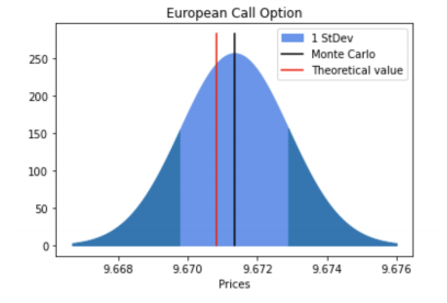
where \( N(0,1) \) is the standard Gaussian variable. Then by randomly generating samples \( ϵ \) from \( N(0,1) \) , we would obtain a discrete stock path by substituting all \( ϵ \) in to the above equation at each time points. We do these above steps \( M \) times to get \( M \) many stock paths. Then we specify the payoff function of the particular option, if it only depends on the final price(i.e Vanilla option) then only final price is needed, if it is a pathdependent option then we have to consider all the time points(i.e Asian option). Finally, we compute the payoffs and average over \( M \) samples to get the MC estimator. A clear demonstration of MC simulation is showing in the Algorithm-1 below. Moreover, Figure 1 is a visualization of difference between BS price and MC price and Figure 2 is the stock paths we generated using MC Simulation given \( {S_{0}}=K=100,T=1,r=0.05 \) . In the following section, we will use these parameters to price many Exotic options.

2. Exotic Options

Exotic options are unusual derivatives created by financial engineers. They may grant the holder specific rights, such as the choice to become put or call at any moment before to maturity(i.e Chooser). Additionally, the value of certain exotic options is reliant on the complete history of stock price, as is the case with Asian options, which are valued based on the “average” of stock prices prior to maturity, according to Hall [7]. In this chapter, we’ll introduce a variety of intriguing exotic options and demonstrate how to calculate their prices. To compare with the precise results, we will also find MC estimators.

2.1. Chooser’s Option

Here we name a buyer a chooser, because the buyer has the right to make the final decision whether to become a call option or a put option at a predetermined time, for example, 12 months. The final payoff of chooser option depends on how the holder’s expectation at the decision time. Now suppose \( {T_{0}} \) is the time to decide if the option should be the call option or the put option. The maturity of the option itself is \( T \) , while strike price at \( T \) is \( K \) , then the payoff function \( CH \) of a choose option is:

\( CH({T_{0}})=max(C(T-{T_{0}},{S_{{T_{0}}}},K),P(T-{T_{0}},{S_{{T_{0}}}},K)) (24) \)

Recall “Put-Call Parity”, then we have:

\( \begin{matrix}CH({T_{0}}) & =max(C,C+K{e^{-r(T-{T_{0}})}}-{S_{{T_{0}}}}) \\ & =C+max(0,K{e^{-r(T-{T_{0}})}}-{S_{{T_{0}}}}) \\ & =C+{(K{e^{-r(T-{T_{0}})}}-{S_{{T_{0}}}})^{+}} \\ & =C(T-{T_{0}},{S_{{T_{0}}}},K)+P({T_{0}},{S_{{T_{0}}}},K{e^{-r(T-{T_{0}})}}) \\ \end{matrix} (25) \)

Thus we proved (11). Notice that chooser’s option is equivalent to the portfolio consisting of a call and a put option.

Theorem 2.1 (Price of Chooser). The price of a chooser option at time \( t=0 \) with maturity \( T \) and strike \( K \) is given by:

\( \begin{matrix}CH(0)={S_{0}}(N({d_{1}})-N(-{\hat{d}_{1}}))+K{e^{-rT}}(N(-{\hat{d}_{2}})-N({d_{2}})) \\ {d_{1}}=\frac{ln⁡({S_{0}}/K)+(r+\frac{1}{2}{σ^{2}})T}{σ\sqrt[]{T}},{d_{2}}={d_{1}}-σ\sqrt[]{T} \\ {\hat{d}_{1}}=\frac{ln⁡({S_{0}}/K)+rT+\frac{1}{2}{σ^{2}}{T_{0}}}{σ\sqrt[]{{T_{0}}}},\hat{{d_{2}}}={\hat{d}_{1}}-σ\sqrt[]{{T_{0}}} \\ \end{matrix} (26) \)

where \( {T_{0}}∈ [0,T] \) is the time to make decision.

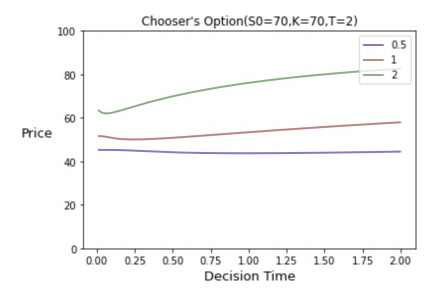
We plot the pricing functions of the Chooser’s options, which we consider as the single-variable function of \( {T_{0}} \) with different \( σ \) , current value \( {S_{0}} \) , strike price \( K \) , interest rate \( r \) and maturity \( T \) (see Figure 3,4 ). If we look at the graph, it’s hard to tell if there’s any useful conclusion we could draw about the monotonicity.

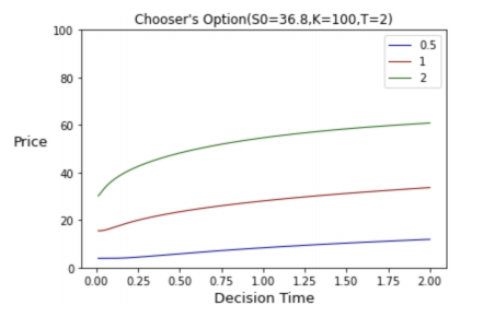
Although it’s intuitive that the price increases in decision time \( {T_{0}} \) , because the closer \( {T_{0}} \) is to \( T \) , the better prediction we might make. However, we should always remember the “discount factor”, which grows exponentially and can “drag down” a significant amount of the price. The following is a theorem including certain criteria for the function to be monotonous increasing:

Theorem 2.2. Under the following conditions, \( CH(0) \) is increasing:

if \( {S_{0}} \gt {e^{-rT}}K \) , then for \( {T_{0}}≥2(ln⁡{S_{0}}/K+rT)/{σ^{2}},CH(0) \) is increasing in \( {T_{0}} \)

if \( {S_{0}}={e^{-rT}}K \) , then \( CH(0) \) monotonously increases

if \( {S_{0}} \lt {e^{-rT}}K \) , then for \( {T_{0}}≤2(ln⁡{S_{0}}/K+rT)/{σ^{2}},CH(0) \) is increasing in \( {T_{0}} \)

Proof. First, \( {S_{0}}={e^{-rT}}K⇔ln⁡{S_{0}}/K+rT=0 \) . According to (12), in the second case \( {\hat{d}_{1}}=\frac{σ\sqrt[]{{T_{0}}}}{2} \) and \( {\hat{d}_{2}}=-\frac{σ\sqrt[]{{T_{0}}}}{2} \) . As error function increases on \( R \) , if \( {T_{0}} \) increases, \( {\hat{d}_{1}} \) increases, so \( N({\hat{d}_{1}}) \) decreases, and \( -{S_{0}}N({\hat{d}_{1}}) \) increases. Similarly, as \( {\hat{d}_{2}} \) decreases in \( {T_{0}},{e^{-rT}}KN(-{\hat{d}_{2}}) \) increases. As a result \( CH(0) \) increases for all \( 0≤{T_{0}}≤T \) .

In the first case, \( {S_{0}} \gt {e^{-rT}}K⇔ln⁡{S_{0}}/K+rT \gt 0 \) . We can rewrite \( {\hat{d}_{1}}=\frac{ln⁡{S_{0}}/K+rT}{σ}\frac{1}{\sqrt[]{{T_{0}}}}+\frac{σ}{2}\sqrt[]{{T_{0}}} \) and \( {\hat{d}_{2}}=\frac{ln⁡{S_{0}}/K+rT}{σ}\frac{1}{\sqrt[]{{T_{0}}}}-\frac{σ}{2}\sqrt[]{{T_{0}}} \) . For \( {\hat{d}_{2}} \) , it’s decreasing because both terms are decreasing. For \( {\hat{d}_{1}} \) , we may know from the fact that the minimum was reached on \( \sqrt[]{{T_{0}}}=\sqrt[]{\frac{ln⁡{S_{0}}/K+rT}{σ}/\frac{σ}{2}}⇔{T_{0}}=2(ln⁡{S_{0}}/K+rT)/{σ^{2}} \) . Thus \( {T_{0}}≥2(ln⁡{S_{0}}/K+rT)/{σ^{2}},CH(0) \) increases. Very similarly, we can prove the third case.

Different price functions converge as the interest rate increases, and in fact we have the following corollary:

Proposition 2.1. As \( r→∞,CH(0)→{S_{0}} \) .

Proof. As \( r→∞,{d_{1}},{d_{2}}→∞ \) , so \( N({d_{1}})→1,N({d_{2}})→0 \) , so the term \( {S_{0}}(N({d_{1}})-N(-{\hat{d}_{1}}))→{S_{0}} \) . As for \( K{e^{-rT}}(N(-{\hat{d}_{2}})-N({d_{2}})),|K{e^{-rT}}(N(-\hat{{d_{2}}})-N({d_{2}}))|≤2|K{e^{-rT}}|→0 \) as \( r→∞ \)

Although “ \( r \) tending to infinity” only exists in theoretical discussion, from Figure 5 we can see that all three curves reach more than 90 when \( r=3 \) .

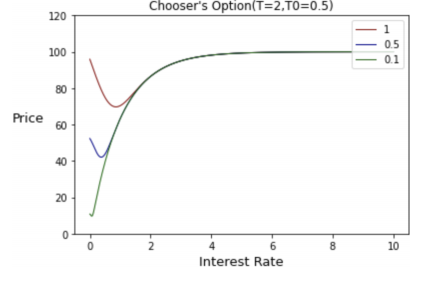
The Monte Carlo Simulation results for Chooser’s Option are demonstrated in Table 1 below, and we take` \( {S_{0}}=K=100,T=1,r=0.05,{T_{0}}=0.5 \) .

Table 1. Chooser’s Option with \( σ=0.5 \)

From Figure 6, also from Table 1, we can also discover that when \( r \) is small, the price of Chooser’s option is decreasing in \( r \) but then increase as \( r \) increases.

2.2. Barrier Option

Barrier option is very similar to European option, but there are upper and lower bounds, which are called barriers. During the whole process, every time when the stock price “hit” the barriers in some ways, the option will be terminated before the maturity.

Here we introduce the down-and-out barrier, and the analysis of other types of barrier option is quite similar. The pay-off function is exactly the European pay-off function, unless the stock price hit a lower bound, which results in the pay-off to be 0. Thus, to let the option reach the maturity. \( {S_{t}} \gt X,∀t∈ [0,T] \) , where \( T \) is the final time. If it goes to the end without hitting the bound, the value is equal to European option \( {({S_{T}}-K)^{+}} \) , and price process \( B(s,t) \) satisfies equation (5) :

\( { B_{t}}(s,t)+rs{B_{s}}(t,s)+\frac{1}{2}{σ^{2}}{s^{2}}{B_{s}}s(t,s)-rB(t,s)=0, for s∈(x,∞) and t∈ [0,T]. (27) \)

However, in the setting of barrier option, the pde has different boundary conditions from European option:

\( \begin{matrix}B(s,K)=s as s→∞ \\ B(X,t)=0 \\ \end{matrix} (28) \)

Now we consider the following series of change of variables:

\( s=K{e^{x}},t=T-2τ/{σ^{2}},B=K{e^{αx+βτ}}u(x,τ) (29) \)

with \( α=-\frac{1}{2}({k_{1}}-1),β=-\frac{1}{4}{({k_{1}}+1)^{2}} \) and \( {k_{1}}=2r/{σ^{2}} \) . Suprisingly, the PDE becomes:

\( \frac{∂u}{∂τ}=\frac{{∂^{2}}u}{∂{x^{2}}} (30) \)

Following the method of images, in Wilmott and Dewynne [9], the final solution to \( B(s,t) \) is

\( B(s,t)=C(s,t)-{(\frac{s}{X})^{-\frac{2r}{{σ^{2}}}+1}}C(\frac{{X^{2}}}{s},t) (31) \)

Here \( C \) is the solution to the normal European call option and:

\( \begin{matrix}C(s,t)=sN({d_{1}}(t,s))-{e^{r(T-s)}}N({d_{2}}(t,s)) \\ {d_{1}}=\frac{(r+{σ^{2}}/2)(T-t)+ln⁡(s/K)}{σ\sqrt[]{T-t}},{d_{2}}=\frac{(r-{σ^{2}}/2)(T-t)+ln⁡(s/K)}{σ\sqrt[]{T-t}} \\ \end{matrix} (32) \)

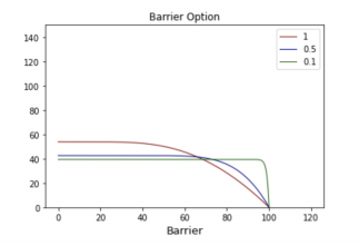
Consider a down-and-out option and let \( {S_{0}}=K=100,X=80 \) .

With other parameters fixed, if we consider the price of Barrier’s option as a single-variable function of the barrier \( X \) : We have an obvious observation:

Proposition 2.2. For a down-and-out barrier option, if the barrier \( X→0 \) , the limit of barrier option is, in fact, its corresponding European call option.

Proof.

1) If \( -\frac{2r}{{σ^{2}}}+1 \lt 0 \) , then we can re-write \( B(s,t) \) as \( B(s,t)=C(s,t)-{(\frac{X}{s})^{\frac{2r}{{σ^{2}}}-1}}C({X^{2}}/s,t) \) . Because \( \frac{2r}{{σ^{2}}}-1 \gt 0 \) , while both \( \frac{X}{s} \) and \( C({X^{2}}/s,t) \) tend to zero at the same time, \( B(s,t)→C(s,t) \) .

2) If \( -\frac{2r}{{σ^{2}}}+1=0,B(s,t)=C(s,t)-C({X^{2}}/s,t)→C(s,t) \) .

3) If \( -\frac{2r}{{σ^{2}}}+1 \gt 0 \) , then we can rewrite the second term in \( B(s,t) \) as \( \frac{C(\frac{{X^{2}}}{s},t)}{\frac{X}{s}-\frac{2r}{{σ^{2}}}+1} \) . Because both \( \frac{X}{s} \) and \( C(\frac{{X^{2}}}{s},t)→0 \) as \( x→0 \) , by applying L’Hopital’s rule for adequate times, we can see \( B(s,t)→C(s,t) \) .

Although we didn’t include up-and-out option, it’s reasonable to expect that if the upper barrier \( X→∞ \) , then \( B(s,t)→C(s,t) \) .

In Table 2 & Table 3, we demonstrated the results for Monte Carlo method, time steps \( =1000 \) , simulations \( =8000 \) and for Binomial model, time steps \( =10000 \) . The results of our simulation is very close to the corresponding analytic solution. In the table below, We compare the results of Monte Carlo with different simulations to the analytical solution.

Table 2. σ=0.25

Table 3. σ=1

2.3. Look-back option

In this section, we give a gentle introduction of Look-back option. Similar to the cases introduced above, all three of them are not path independent. However notice that in the previous cases, the investors they can only view the price progression at maturity, according to Bingham and Kiesel [10]. The right to sell a stock at the highest point is provided by a lookback put option, while the ability to purchase a stock at the lowest point is provided by a lookback call option. Let \( LC,LP \) denotes the payoff of lookback call and lookback put options respectively, then:

\( \begin{matrix} & LC(T)={({S_{T}}-\underset{0≤u≤T}{min} {S_{u}})^{+}}={S_{T}}-\underset{0≤u≤T}{min} {S_{u}} \\ & LP(T)={(\underset{0≤u≤T}{max} {S_{u}}-{S_{T}})^{+}}=\underset{0≤u≤T}{max} {S_{u}}-{S_{T}} \\ \end{matrix} (33) \)

Note the payoff for a Lookback option is always non-negative. According to the risk-neutral valuation formula, the price of a Lookback option at time \( t∈ [0,T] \) is :

\( \begin{matrix}LC(t) & ={e^{-r(T-t)}}E[{S_{T}}-\underset{0≤u≤T}{min} {S_{u}}∣{F_{t}}] \\ & ={e^{-r(T-t)}}E[{S_{T}}∣{F_{t}}]-{e^{-r(T-t)}}E[\underset{0≤u≤T}{min} {S_{u}}∣{F_{t}}] (34) \\ & ={S_{t}}-{e^{-r(T-t)}}E[\underset{0≤u≤T}{min} {S_{u}}∣{F_{t}}] \\ \end{matrix} \)

Given the information \( {F_{t}} \) , we know exactly the stock price evolution before time \( t \) . Therefore, let \( m=min({S_{u}} \) : \( 0≤u≤t) \) be the minimum point in the history of the stock. Then, \( \underset{0≤u≤T}{min} {S_{u}}=min(m,\underset{t≤u≤T}{min} {S_{u}}) \) , where \( \underset{t≤u≤T}{min} {S_{u}} \) is independent with \( {F_{t}} \) . For convenience, let \( τ=T-t,{λ^{±}}=r±\frac{{σ^{2}}}{2} \) and recall that for any \( u∈ [t,T] \) , we have:

\( {S_{u}}={S_{t}}{e^{σ({W_{u}}-{W_{t}})+{λ^{-}}(u-t)}}={S_{t}}{e^{-({X_{u}}-{X_{t}})}} (35) \)

where \( {X_{u}}=-σ{W_{u}}-{λ^{-}}u \) , then:

\( \underset{t≤u≤T}{min} {S_{u}}={S_{t}}{e^{-\underset{t≤u≤T}{max} ({X_{u}}-{X_{t}})}}={S_{t}}{e^{-\underset{0≤u≤τ}{max} {X_{u}}}} (36) \)

Hence:

\( \begin{matrix}LC(t) & ={S_{t}}-{e^{-r(T-t)}}E[min(m,\underset{t≤u≤T}{min} {S_{u}})] \\ & ={S_{t}}+m-{e^{-r(T-t)}}E[min(0,\underset{t≤u≤T}{min} {S_{u}}-m)] \\ & ={S_{t}}+m-{e^{-r(T-t)}}E[({S_{t}}exp⁡(-\underset{0≤u≤τ}{max} {X_{u}})-m){1_{(max{X_{u}}≥-ln⁡(\frac{m}{{S_{t}}}))}}] \\ \end{matrix} (37) \)

Then we are left to compute \( P((max{X_{u}}≥-ln⁡(\frac{m}{{S_{t}}})) \) . Musiela and Rutkowsk [7] solved this problem using reflection principle and their results are:

\( LC(t)={S_{t}}N({d_{1}})-m{e^{-rτ}}N({d_{2}})-\frac{{S_{t}}{σ^{2}}}{2r}N(-{d_{1}})-{e^{-rτ}}\frac{{S_{t}}{σ^{2}}}{2r}{(\frac{m}{{S_{t}}})^{2r{σ^{-2}}}}N({d_{3}}) (38) \)

where:

\( {d_{1}}=\frac{ln⁡(\frac{{S_{t}}}{m})+{λ^{+}}τ}{σ\sqrt[]{τ}},{d_{2}}={d_{1}}-σ\sqrt[]{τ},{d_{3}}=\frac{2r\sqrt[]{τ}}{σ}-{d_{1}} (39) \)

For Lookback put option:

\( LP(t)=-{S_{t}}N(-{d_{1}})+M{e^{-rτ}}N(-{d_{2}})+\frac{{S_{t}}{σ^{2}}}{2r}N({d_{1}})-{e^{-rτ}}\frac{{S_{t}}{σ^{2}}}{2r}{(\frac{m}{{S_{t}}})^{2r{σ^{-2}}}}N(-{d_{3}}) (40) \)

where \( M=\underset{0≤u≤T}{max} {S_{u}} \) is a fixed number under \( {F_{t}} \) . The Monte Carlo results are shown in Table 4, with \( S=K=100 \)

Table 4. Lookback option with different σ

2.4. Asian Option

Different from the options we introduced above, Asian options take the value of the stock price throughout the period by taking the “average”. There are different ways to take the average, but in our context, we only introduce the arithmetic Asian option. For arithmetic Asian option, we also have the following two sub-categories, which is defined based on whether the strike price is fixed:

\( \begin{matrix}E{(\frac{1}{T}\int _{0}^{T}  {S_{u}}du-K)^{+}}(Fixed Strike)  \\ E{(\frac{1}{T}\int _{0}^{T}  {S_{u}}du-{S_{T}})^{+}}(Floating Strike)  \\ \end{matrix} (40) \)

2.5. Method of Rogers and Shi

According to Rogers and Shi [11], for fixed Asian option, the definition of function \( ϕ \) is extremely helpful in the following derivation of the price function of Asian option. Define:

\( ϕ(t,x):=E{(\frac{1}{T}\int _{t}^{T}  {S_{u}}du-x)^{+}} (41) \)

Notice that we can interpret \( ϕ(t,x) \) to be the function reflecting the payoff of the option at maturity with respect to its value at time \( t \) . In this paper, the significance of their work is the success to reduce the previous two space dimension pde corresponding to Asian fixed price to one space dimension pde.

Theorem 2.3. Define:

\( {M_{t}}:=E({(\frac{1}{T}\int _{0}^{T}  {S_{u}}du-K)^{+}}∣{F_{t}}) (42) \)

where \( {F_{t}} \) represents all the information about stock price until time \( t \) . Then \( {M_{t}} \) is a martingale and

\( {M_{t}}={S_{t}}ϕ(t,{ξ_{t}}), {ξ_{t}}=\frac{K-\frac{1}{T}\int _{0}^{t}  Sudu}{{S_{t}}} (43) \)

Proof. Let \( t≥s \) , then it’s immediate that \( {F_{s}}⊆{F_{t}} \) . Also we see that

\( \begin{matrix}E({M_{t}}∣{F_{s}}) & =E[(E({(\frac{1}{T}\int _{t}^{T}  {S_{u}}du-K)^{+}}∣{F_{t}}))∣{F_{s}}] \\ & =E({(\frac{1}{T}\int _{t}^{T}  {S_{u}}du-K)^{+}}∣{F_{s}})  (by Tower property)  \\ & ={M_{s}} \\ \end{matrix} (44) \)

Thus by previous calculation, \( {M_{t}} \) is a martingale. To see the second property holds:

\( \begin{matrix}{M_{t}}: & =E({(\frac{1}{T}\int _{0}^{T}  {S_{u}}du-K)^{+}}∣{F_{t}}) \\ & =E[{(\frac{1}{T}\int _{t}^{T}  {S_{u}}du-(K-\frac{1}{T}\int _{0}^{t}  {S_{u}}du))^{+}}∣{F_{t}}] \\ & ={S_{t}}E[{(\frac{1}{T}\int _{t}^{T}  \frac{{S_{u}}}{{S_{t}}}du-\frac{K-\frac{1}{T}\int _{0}^{t}  {S_{u}}du}{{S_{t}}})^{+}}∣{F_{t}}] \\ \end{matrix} (45) \)

As \( {ξ_{t}} \) is a deterministic function of \( {S_{u}}, ∀u∈ [0,t] \) , and \( {S_{u}} \) is \( {F_{{t^{-}}}}measurable by construction, {ξ_{t}} \) is \( {F_{{t^{-}}}} \) measurable. Thus \( {ξ_{t}} \) is \( {F_{t}} \) -measurable. This means that given information of \( {F_{t}},{ξ_{t}} \) is fixed instead of a random variable, so we can let \( x={ξ_{t}} \) .

In view of Black-Scholes’ model, it’s clear that \( {S_{u}}={S_{t}}exp⁡\lbrace σ({W_{u}}-{W_{t}})\rbrace +(r-\frac{{σ^{2}}}{2}(u-t)\rbrace \) . If \( {S_{t}} \) is fixed, then \( \frac{{S_{u}}}{{S_{t}}} \) is independent of \( {F_{t}} \) , as \( {W_{u}}-{W_{t}} \) is independent of \( {F_{t}} \) . Thus we have:

\( \begin{matrix}{M_{t}} & ={S_{t}}E{(\frac{1}{T}\int _{t}^{T}  \frac{{S_{u}}}{{S_{t}}}du-{ξ_{t}})^{+}}∣{F_{t}}] \\ & ={S_{t}}E{(\frac{1}{T}\int _{t}^{T}  \frac{{S_{u}}}{{S_{t}}}du-{ξ_{t}})^{+}} \\ & ={S_{t}}ϕ(t,{ξ_{t}}) \\ \end{matrix} (46) \)

Theorem 2.4 (A PDE approach). Let \( f={e^{-r(T-t)}}ϕ(t,x) \) represents the price of Asian option. Then \( f(t,x) \) is determined by the following partial differential equation :

\( \frac{df}{dt}+\frac{1}{2}{σ^{2}}{x^{2}}\frac{{d^{2}}f}{d{x^{2}}}=(\frac{1}{T}+rx)\frac{df}{dx} (48) \)

With boundary conditions at \( t=T \) :

\( \begin{matrix}f(T,x)=-max(x,0)( Fixed Strike ) \\ f(T,x)=-max(1+x,0)( Floating Strike ) \\ \end{matrix} (49) \)

and when \( x \lt =0 \) :

\( \begin{matrix}f(t,x)=\frac{(1-{e^{-r(T-t)}}){S_{t}}}{rT}-x{e^{-r(T-t)}}(Fixed Strike) \\ f(t,x)=\frac{(1-{e^{-r(T-t)}}){S_{t}}}{rT}-x{e^{-r(T-t)}}-{S_{t}}(Floating Strike) \\ \end{matrix} (50) \)

Proof. (Sketch) The idea of the proof is to apply the Ito product rule to \( {M_{t}} \) . Since \( {M_{t}} \) is a function of \( {S_{t}} \) and \( ϕ,ϕ \) is also a function of \( t \) and \( ξ \) . Therefore, we have to find the corresponding stochastic differential equation for each of them. Then according to the properties of martingale \( {M_{t}} \) , when obtain the PDE. We will only prove the case when strike price is fixed, the proof for floating strike is similar.

Recall \( {ξ_{t}}=\frac{1}{{S_{t}}}(K-\frac{1}{T}\int _{0}^{t}  {S_{u}}du)=-\frac{1}{{S_{t}}}{A_{t}} \) where

\( \begin{matrix} & d({A_{t}})=d(K-\frac{1}{T}\int _{0}^{t}  {S_{u}}du)=\frac{1}{T}{S_{t}}dt \\ \end{matrix} (51) \)

Apply Ito chain rule to \( {Y_{t}}=\frac{1}{{S_{t}}} \) :

\( \begin{matrix}d{Y_{t}}=d\frac{1}{{S_{t}}} & =(0-\frac{1}{S_{t}^{2}}r{S_{t}}+\frac{1}{2}\frac{2}{S_{t}^{3}}{σ^{2}}S_{t}^{2})dt-σ{S_{t}}\frac{1}{S_{t}^{2}}dW \\ & =-\frac{1}{{S_{t}}}(r-{σ^{2}})dt-\frac{1}{{S_{t}}}σdW \\ \end{matrix} (52) \)

Then apply Ito product rule:

\( \begin{matrix}d{ξ_{t}} & ={A_{t}}d(\frac{1}{{S_{t}}})+\frac{1}{{S_{t}}}d{A_{t}}+d(\frac{1}{{S_{t}}})d{A_{t}} \\ & =(K-\frac{1}{T}\int _{0}^{t}  {S_{u}}du)(-\frac{1}{{S_{t}}}(r-{σ^{2}})dt-\frac{1}{{S_{t}}}σdW)-\frac{1}{{S_{t}}}\frac{1}{T}{S_{t}}dt \\ & =-{ξ_{t}}(r-{σ^{2}})dt-{ξ_{t}}σdW-\frac{1}{T}dt \\ & =(-\frac{1}{T}-{ξ_{t}}r+{ξ_{t}}{σ^{2}})dt-σ{ξ_{t}}dW \\ \end{matrix} (53) \)

Then apply Ito chain rule to \( ϕ(t,ξ) \) :

\( dϕ=(\dot{ϕ}+(-\frac{1}{T}-ξr+ξ{σ^{2}}){ϕ^{ \prime }}+\frac{1}{2}{σ^{2}}{ξ^{2}}{ϕ^{ \prime \prime }})dt-σξ{ϕ^{ \prime }}dW (54) \)

Since \( {M_{t}} \) is a function of \( {S_{t}} \) and \( ϕ \) , so the Ito product rule gives the following :

\( \begin{matrix}dM & =ϕdS+Sdϕ+dSdϕ \\ & =ϕ(rSdt+σSdW)+S((ϕ+(-\frac{1}{T}-ξr+ξ{σ^{2}}){ϕ^{ \prime }}+\frac{1}{2}{σ^{2}}{ξ^{2}}{ϕ^{ \prime \prime }})dt-σξ{ϕ^{ \prime }}dW)-{σ^{2}}{S_{t}}ξ{ϕ^{ \prime }}dt \\ & =S(rϕ+\dot{ϕ}+{ϕ^{ \prime }}(-\frac{1}{T}-rξ)+\frac{{σ^{2}}}{2}{ξ^{2}}{ϕ^{ \prime \prime }})dt+(ϕσS-{ϕ^{ \prime }}σξS)dW \\ \end{matrix} (55) \)

We have shown that \( {M_{t}} \) is a martingale, so the “ \( dt \) “ term in the corresponding SDE must be 0 , hence we get:

\( \begin{matrix}rϕ+\dot{ϕ}+{ϕ^{ \prime }}(-\frac{1}{T}-rξ)+\frac{{σ^{2}}}{2}{ξ^{2}}{ϕ^{ \prime \prime }}=0 \\ rϕ+\dot{ϕ}+\frac{{σ^{2}}}{2}{ξ^{2}}{ϕ^{ \prime \prime }}={ϕ^{ \prime }}(\frac{1}{T}+rξ) \\ \end{matrix} (56) \)

Recall \( f={e^{-r(T-t)}}ϕ(t,x) \) , so \( \frac{df}{dt}=rϕ+\dot{ϕ} \) , and hence:

\( \frac{df}{dt}+\frac{1}{2}{σ^{2}}{x^{2}}\frac{{d^{2}}f}{d{x^{2}}}=(\frac{1}{T}+rx)\frac{df}{dx} (57) \)

Therefore, the price of Asian option is given by \( f(0,KS_{0}^{-1}) \) . For boundary conditions:

At \( t=T: \) \( f(T,x)=ϕ(T,x)=E[{(\frac{1}{T}\int _{T}^{T}  {S_{u}}du-x)^{+}}]=-(x{)^{+}}=min(x,0) (58) \)

When \( x≤0 \) :

\( \begin{matrix}f(t,x) & ={e^{-r(T-t)}}E[{(\frac{1}{T}\int _{t}^{T}  {S_{u}}du-x)^{+}}] \\ & ={e^{-r(T-t)}}\frac{1}{T}\int _{t}^{T}  E[{S_{u}}]du-x{e^{-r(T-t)}} \\ & ={e^{-r(T-t)}}\frac{1}{T}\int _{t}^{T}  {S_{t}}{e^{r(u-t)}}du-x{e^{-r(T-t)}} \\ & ={e^{-r(T-t)}}\frac{{S_{t}}}{T}({e^{r(T-t)}}-1)-x{e^{-r(T-t)}} \\ & =\frac{(1-{e^{-r(T-t)}}){S_{t}}}{rT}-x{e^{-r(T-t)}} \\ \end{matrix} (59) \)

Although, it’s very difficult to obtain a general expression of the price function using the PDE (for positive \( x \) for example), Roger and Shi provided an effective way to check the lower bounds for price functions.

Theorem 2.5 (Roger and Shi Lower Bound). \( X \) is a random variable such that \( X=\frac{1}{T}∫_{0}^{T} {S_{T}}-K.X \) can be split into a positive part \( {X^{+}} \) and a negative part \( {X^{-}} \) such that \( X={X^{+}}-{X^{-}} \) and :

\( \begin{matrix}E({X^{+}})=E(E(X∣{Z^{+}}))≥E(E(X∣Z{)^{+}}) \\ 0≤E({X^{+}})-E(E(X∣Z{)^{+}})≤\frac{1}{2}E(\sqrt[]{Var⁡(X∣Z)}) \\ \end{matrix} (60) \)

Therefore, we have the lower and upper bound for the payoff function of Asian option :

\( \begin{matrix}LB=E(E(X∣Z{)^{+}}) \\ UB=E(E(X∣Z{)^{+}})+\frac{1}{2}E(\sqrt[]{Var⁡(X∣Z)}) \\ \end{matrix} (61) \)

where \( Z \) is a Gaussian process with mean 0.

Table 5 demonstrates the results of Monte Carlo Simulations together with the numerical method data from Roger and Shi’s paper. In fact, we can see that Monte Carlo Simulation gets more accurate information than the numerical methods used by Roger and Shi.

Table 5. Asian option with different σ

3. Conclusion

This paper starts from introducing the built-up of Continuous time model to show two approaches to get an option pricing formula. One is using the Risk-Neutral Valuation formula directly compute the expectation of the payoff function under risk-neutral measure. The other is to use the replicating portfolio for an option, then by law of one price they must have the same initial values. In the second method, we will end up a PDE with some boundary conditions whose solution(may be analytic or numeric) is the price of that option. We start from a simple example, the chooser option. After discussing about its feature, we found that its payoff is just the sum of a call and a put option, thus the price formula is straightforward. For Barrier option, we found it is easy to solve the corresponding PDE. For Look-back option, the risk neutral valuation formula works nicely, it was easy to get a explicit solution using reflection principle. Asian option is the most complicated example in our paper. We reviewed Roger and Shi’s method to derive and solve the embedded PDE together with the lower bound method.

For each exotic option, we also compute the MC estimator for their price and compare with the exact solution. Our results show that Monte Carlo is a very reliable approximation, especially when we have a strong machine. For example, in Table 4, when we take N=10000, with M=10⁶, the errors of Monte Carlo Simulation never go above 2%. Also, for example, in Table 5, the Monte Carlo simulation is much more reliable than the numerical solution to the partial differential equation derived by Roger and Shi. Moreover, although as in Table 3, binomial model is already a very good approximation to the analytic solution of the Barrier Option, the program of binomial model is always one-dimensional but the Monte Carlo Simulation allows multi-dimensions.

References

[1]. Akyıldırım, E., Soner, H. (2014). A brief history of mathematics in finance. Borsa Istanbul Review, 14(1): 57-63.
[2]. Yan, J., (2022) Martingale Approach to Option Pricing. [online] Ims.cuhk.edu.hk. http://www.ims.cuhk.edu.hk/conference/june99/yanabs.html
[3]. Evans, L. (2014). An Introduction to Stochastic Differential Equations American Mathematical Society: Washington D.C.
[4]. Black, F., Scholes, M. (1973) The Pricing of Options and Corporate Liabilities. Journal of Political Economy, 81(3): 637-654.
[5]. Musiela, M., Rutkowski, M. (2010). Martingale methods in financial modelling. Springer, Berlin.
[6]. Saari, D. (2019). Mathematics of finance. Springer, Cham.
[7]. Hull, J. (2014) Options, futures, and other derivatives. Prentice Hall, Upper Saddle River.
[8]. Bendob, A., Bentouir, N., (2019). Options Pricing by Monte Carlo Simulation, Binomial Tree and BMS Model: a comparative study of Nifty50 options index. Journal of Banking and Financial Economics, 1/2019(11): 79-95.
[9]. Wilmott, P., Dewynne, J., Howison, Sam., (1994). Oxford Financial Press, New York.
[10]. Bingham, N., Kiesel, R. (2004) Risk-Neutral Valuation. Springer London, London.
[11]. Rogers, L., Shi, Z. (1995). The value of an Asian option. Journal of Applied Probability, 32(04): 1077-1088.
Cite this article
Lu,Y.;Zhang,H. (2024). Exotic options pricing in continuous time with Monte Carlo simulations. Theoretical and Natural Science,34,315-329.
Data availability
The datasets used and/or analyzed during the current study will be available from the authors upon reasonable request.
Disclaimer/Publisher's Note
The statements, opinions and data contained in all publications are solely those of the individual author(s) and contributor(s) and not of EWA Publishing and/or the editor(s). EWA Publishing and/or the editor(s) disclaim responsibility for any injury to people or property resulting from any ideas, methods, instructions or products referred to in the content.
About volume
Volume title: Proceedings of the 3rd International Conference on Computing Innovation and Applied Physics
© 2024 by the author(s). Licensee EWA Publishing, Oxford, UK. This article is an open access article distributed under the terms and
conditions of the Creative Commons Attribution (CC BY) license. Authors who
publish this series agree to the following terms:
1. Authors retain copyright and grant the series right of first publication with the work simultaneously licensed under a Creative Commons
Attribution License that allows others to share the work with an acknowledgment of the work's authorship and initial publication in this
series.
2. Authors are able to enter into separate, additional contractual arrangements for the non-exclusive distribution of the series's published
version of the work (e.g., post it to an institutional repository or publish it in a book), with an acknowledgment of its initial
publication in this series.
3. Authors are permitted and encouraged to post their work online (e.g., in institutional repositories or on their website) prior to and
during the submission process, as it can lead to productive exchanges, as well as earlier and greater citation of published work (See
Open access policy for details).