1 Introduction

The normal distribution, also known as the Gaussian distribution, is a widely observed and important concept in many fields. It is a probability distribution that describes the probability of various events occurring within a given range. The normal distribution applies to various phenomena, such as measurement error, the distribution of impact points of artillery shells, human physiological features (such as height and weight), crop harvests, and more. These observations approximately follow the normal distribution, making them a useful tool for measuring and predicting outcomes. Theoretically, the normal distribution (Gaussian distribution) is an important probability distribution in mathematics, physics, engineering, and other fields. The normal distribution has a significant impact on many aspects of statistics. It is commonly used to test hypotheses, to make predictions, and to estimate parameters. The normal distribution is also used to model the behavior of many natural phenomena, such as the movement of particles in a gas or the spread of a disease [1]. This paper sets out to solve the secrets of the normal distribution, investigating its definition, intrinsic features, historical beginnings, evolution, and many ramifications for the actual world.

2 Definition of the Normal Distribution

The normal distribution, sometimes known as the Gaussian distribution, is a probability distribution used extensively in mathematics, physics, and engineering. It has a huge impact on many areas of statistics. If a random variable has a probability distribution that includes both a location and a scale parameter, its probability density function is the mathematical expectation of the normal distribution. The expected value, which determines the distribution’s position, equals the location parameter. The open square of its variance, or standard deviation, equals the scale parameter, which determines the distribution’s magnitude [2].

If the probability density function of a continuous random variable \( X \) is:

\( f(x)=\frac{1}{σ\sqrt[]{2π}}e^{\frac{-(x-u)^{2}}{2σ^{2}}} \) , \( x∈(-∞,+∞) \) (1)

where \( μ, σ (σ \gt 0) \) are constants, Then \( X \) is said to follow a normal or Gaussian distribution with parameters \( μ, σ^{2} \) , denoted by \( X~N(μ,σ^{2}) \) . If \( μ=0, σ=1 \) , Then \( X \) is said to follow a standard normal distribution with a probability density function of

\( ∅(x)=\frac{1}{\sqrt[]{2π}}e^{\frac{-x^{2}}{2}} \) , \( x∈(-∞,+∞) \) (2)

The distribution functions for the general normal and standard normal distributions are:

\( F(x)=\int_{-∞}^{x} \frac{1}{σ\sqrt[]{2π}}e^{-\frac{(t-μ)^{2}}{2σ^{2}}}dt, xϵ(-∞,+∞) \) (3)

\( ∅(x)=\int_{-∞}^{x} \frac{1}{\sqrt[]{2π}}e^{-\frac{t^{2}}{2}}dt, xϵ(-∞,+∞) \) (4)

3 Attributes of the Normal Distribution

The normal distribution has a number of important attributes [3]:

The image of a normal distribution probability density \( f(x) \) is a bell-shaped, single-peaked function symmetric about \( X=μ \) . \( f(x) \) obtains a maximum value of \( \frac{1}{σ\sqrt[]{2π}} \) at \( X=μ \) . The further away \( X \) is from \( μ \) , the smaller the value of \( f(x) \) , which indicates that for intervals of the same length, the farther away from \( μ \) the interval is, the smaller the probability is that \( X \) will fall on this interval.

At \( x=μ±σ \) , the curve \( y=f(x) \) has inflection points at the corresponding points. In addition, if \( σ \) is fixed and the value of \( μ \) is changed, the graph translates along the \( Qx \) without changing its shape (as shown in Figure 1). The position of the probability density curve \( y=f(x) \) of the normal distribution is ultimately determined by the parameter \( μ \) , and the fixed \( μ \) is known as the position parameter.

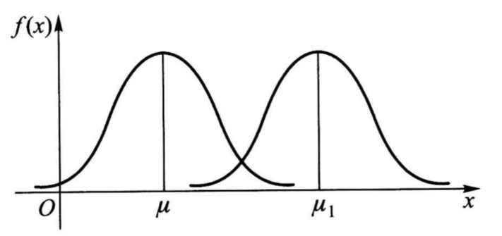
Figure 1. Probability Density Function of Two Different Parameters

\( μ \) -positional parameter, i.e., fixing \( μ \) , for different \( σ \) , \( f(x) \) has different shapes. Since the maximum value \( f(μ)=\frac{1}{σ\sqrt[]{2π}} \) , the graph becomes sharper when \( σ \) is more minor (as shown in Figure 2), and thus the probability that \( X \) falls near \( μ \) is higher.

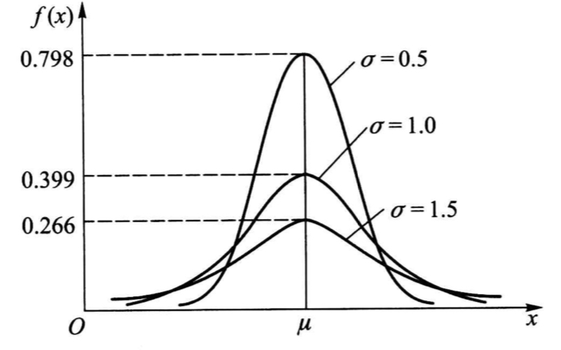
Figure 2. Probability Density Function of Three Different Parameters

According to the characteristics of the probability density \( f(x) \) image of a normal distribution and the geometric significance of the distribution function of a random variable, \( P(X≤μ)=P(X≥μ)=0.5 \) , \( ϕ(0)=0.5 \) , \( ϕ(-x)=1-ϕ(x) \) . (as in Figure 3)

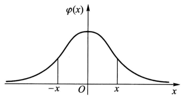
Figure 3. Probability Density Function

4 Origin and Development of the Normal Distribution

The concept of the normal distribution was first proposed by Abraham de Moivre, a German mathematician and astronomer, in 1733. Still, the normal distribution is also known as the Gaussian distribution because Gauss, a German mathematician, was the first to apply it to astronomers’ research. Thus, later generations attribute the invention of the least squares method to him [4]. Nowadays, the German 10-mark banknote featuring Gauss’s head also displays the density curve of the normal distribution, highlighting the significant impact of his scientific contributions on human civilization. This shows that Gauss’s scientific contributions had a significant impact on human civilization. At the beginning of the discovery of the normal distribution, its superiority could only be evaluated from the simplification of its theory, and its full impact could not be fully seen. It was not until the theory of standard small samples was fully developed in the twentieth century that Pierre-Simon Laplace quickly learned of Gauss’s work and immediately connected it to his discovery of the Central Limit Theorem, to which he added in a forthcoming article (published in 1810) that if the error can be viewed as a superposition of many quantities, the error should have a Gaussian distribution [5]. This was the first historical reference to the so-called “meta-error doctrine”, which suggests errors are the result of the superposition of many meta-errors arising from a variety of causes - which was formally introduced in a paper by G. Hagen in 1837 [6].

In fact, the form of his proposal has considerable limitations: Hagen conceived the error as many independently and identically distributed “meta-errors” sum, each of which takes two values, the probability of which is 1/2, from which, according to the central limit theorem of A. de. Moivre, it is immediately concluded that the error (approximately) obeys a normal distribution. The statement made by Pierre-Simon Laplace is crucial because he provides a more naturally rational and persuasive interpretation of the normal theory of error. Gauss used a circular argument: because the arithmetic mean is excellent, the error must follow a standard distribution, and the latter conclusion leads to the excellence of the arithmetic mean and the least squares estimate, so one of these two (arithmetic mean excellence or error normality) must be recognized as the starting point. However, the arithmetic mean cannot stand on its own, and adopting it as a presumptive starting point in the theory has limitations. Laplace’s logic is important in resolving this broken connection and creating a harmonic whole.

5 Applications of the Normal Distribution

5.1 Estimation of the Frequency Distribution of Normally Distributed Information

In real life, when statistical methods are used to analyze data over a period of time, it is necessary to understand the distribution of certain data on the whole. If the distribution of the whole data at this time conforms to the standard curve, it is possible to carry out relatively simple calculations through the normal distribution, using a one-step normal distribution in the transformation between the standard normal distribution and then look up the table. For example, some scholars have carried out statistical tests on the frequency of monthly precipitation in Shanxi Province and concluded that the annual rainfall complies with the normal distribution, and the monthly rainfall, after doing the cube root transformation, complies with the normal distribution in 83% of the stations and months, and so on [7].

5.2 Survey on the Students’ Situation

Students’ performance has always been a common concern of society, which brings about the development of educational statistics. According to the analysis of the statistical results of many students, the student’s intelligence level, ability to learn and innovate, and acceptance of new things align with the standard curve. Of course, the distribution of students’ scores is even more typical of a normal distribution. Students’ test scores are more concentrated around a specific score, and the number of high and low scores is relatively small. If the curve is relatively flat or more skewed to a particular side, obviously asymmetrical, then this examination’s situation may be abnormal [8].

5.3 Designation of Medical Reference Value Ranges

The fluctuation range of specific indicators for most ordinary people is called the expected value range of the indicator. Ordinary people do not mean people without disease, but this indicator does not affect the results under certain conditions. Many indicators, such as a person’s height, the number of red and white blood cells, etc., have a standard or approximately normal distribution. Some indicators do not fully obey the normal distribution, such as when the new variables follow the normal distribution after a simple transformation of the data [9].

5.4 Theoretical Foundations of Statistical Methods

In probability theory, the t distribution and F distribution are based on the normal distribution; the formation of the u test is also very much related to the normal distribution. In addition, the limit of the t distribution, binomial distribution, and Poisson distribution for normal distribution, under certain conditions, can be handled according to the principle of normal distribution [10].

6 Conclusion

Defined by its probability density function, the normal distribution is characterized by its bell-shaped curve, symmetric around its mean, with probabilities decreasing as the distance from the mean increases. Its parameters, including the mean ( \( μ \) ) and standard deviation ( \( σ \) ), play crucial roles in determining the distribution’s location and spread. Originating from the works of Abraham de Moivre and further developed by Gauss and Laplace, the normal distribution has become central to statistical theory. Laplace’s insight into the connection between errors and normal distribution paved the way for its widespread adoption in statistical analysis. In practical applications, the normal distribution serves as a powerful tool for estimating frequency distributions, such as in analyzing precipitation data or student performance. It also guides medical practitioners in establishing reference ranges for various physiological indicators. Furthermore, the normal distribution underpins many statistical methods, including hypothesis testing and parameter estimation.

In conclusion, the versatility, elegance, and real-world applicability of normal distribution underscore its enduring importance in both theoretical and practical contexts. The understanding of randomness and uncertainty has advanced knowledge and innovation across disciplines through continuous exploration of their complexity. The exploration of the normal distribution has revealed its profound significance across disciplines and probability theory. From its historical roots to its modern applications, the normal distribution (also known as the Gaussian distribution) has become a cornerstone concept. It describes the probability of an event occurring within a given range and is widely used in fields such as mathematics, physics, engineering, and statistics.

References

[1]. Hu, X. J. (2014). Overview of the Normal Distribution and Its Extensions. Mathematical Learning and Research, (3), 3.
[2]. Sheng, Z. (2001). Probability Theory and Mathematical Statistics: Third Edition. Higher Education Press.
[3]. Yu, N. (2015). Exploration of Learning about the Normal Distribution. Science and Technology Innovation, (34), 90-91.
[4]. Robinson, L. R. (2017). It’s time to move on from the bell curve. Muscle & Nerve, 56(5), 859-860.
[5]. Laplace, P. S. (1814). Théorie analytique des probabilités. Courcier.
[6]. Fischer, H., & Fischer, H. (2011). The Hypothesis of Elementary Errors. A History of the Central Limit Theorem: From Classical to Modern Probability Theory, 75-138.
[7]. Yang, G. Z. (1983). Theoretical Frequency Distribution of Annual and Monthly Precipitation in Shaanxi Province. Plateau Meteorology, V2(2), 36-41.
[8]. Feng, Y. M. (1996). Application of the Normal Distribution in Education. Journal of Sichuan Vocational and Technical College, 006(002), 5-8.
[9]. Wang, X. (2019). Application of the Normal Distribution Model in Medicine. College Entrance Examination, (3), 2.
[10]. Yuan, S. S., Wang, J. L., & Pu, X. L. (1998). Advanced Mathematical Statistics. Springer.
Cite this article
Ye,X. (2024). Unveiling the intricacies of the normal distribution: From theory to applications. Theoretical and Natural Science,36,175-179.
Data availability
The datasets used and/or analyzed during the current study will be available from the authors upon reasonable request.
Disclaimer/Publisher's Note
The statements, opinions and data contained in all publications are solely those of the individual author(s) and contributor(s) and not of EWA Publishing and/or the editor(s). EWA Publishing and/or the editor(s) disclaim responsibility for any injury to people or property resulting from any ideas, methods, instructions or products referred to in the content.
About volume
Volume title: Proceedings of the 2nd International Conference on Mathematical Physics and Computational Simulation
© 2024 by the author(s). Licensee EWA Publishing, Oxford, UK. This article is an open access article distributed under the terms and
conditions of the Creative Commons Attribution (CC BY) license. Authors who
publish this series agree to the following terms:
1. Authors retain copyright and grant the series right of first publication with the work simultaneously licensed under a Creative Commons
Attribution License that allows others to share the work with an acknowledgment of the work's authorship and initial publication in this
series.
2. Authors are able to enter into separate, additional contractual arrangements for the non-exclusive distribution of the series's published
version of the work (e.g., post it to an institutional repository or publish it in a book), with an acknowledgment of its initial
publication in this series.
3. Authors are permitted and encouraged to post their work online (e.g., in institutional repositories or on their website) prior to and
during the submission process, as it can lead to productive exchanges, as well as earlier and greater citation of published work (See
Open access policy for details).