1. Introduction

Due to the increasing demand for travel in today’s life, more and more families are willing to bear the burden of owning a car. Consequently, the demand for the second-hand car market has been continuously rising. For the majority of people, purchasing a second-hand car is more affordable, and second-hand cars are cheaper and more cost-effective. They also facilitate buyers to resell them, thereby reducing expenses or adjusting their demands. Except the factors that influence the prices of second-hand cars in different countries or regions, there are still many factors that can affect the price of a second-hand car, such as mileage, brand, and registration time. In this case, predicting the price of a second-hand car model requires a large amount of transaction data from the second-hand car market to assist.

In fact, there have been several previous studies on predicting second-hand car prices. Monburiono et al. utilized linear regression algorithm, random forest algorithm, and gradient boosted regression trees to analyze nearly 370,000 data points of second-hand cars. They compared the results using mean absolute error as a benchmark and found that the gradient boosted regression trees model yielded the smallest error value, followed by the random forest algorithm. This study utilized a different dataset and attempted to predict the trend of second-hand car prices using various regression algorithms based on machine learning models [1].

Kanwal Noor and Sadaqat Jan used multiple linear regression as the machine learning prediction method, which is suitable for studying the price prediction of the second-hand car market with multiple independent variables and one dependent variable. In the experiment, the author sets the price as the dependent variable and vehicle model, brand, mileage, color, etc. as independent variables to predict vehicle prices. Finally, they compared actual values with predicted values and achieved a high prediction accuracy of 98% [2].

Wang feng et al. used machine learning algorithms to predict the prices of second-hand cars. They first preprocessed the dataset and compared the algorithm performance through algorithm comparison functions. Ultimately, they found that Random Forest Regressor and Extra Trees Regressor performed well, and after optimization, they obtained the final model for predicting second-hand car prices [3]. Janke et al. discovered the issue of fraud in the used car market and proposed a low-error prediction model for curbing such behavior. They constructed an artificial neural network using Keras regression algorithm and machine learning algorithms like random forest. After testing these algorithms on a dataset of car information, they found that the random forest model had the lowest average error. This finding may contribute to the development of a highly accurate second-hand car price prediction model in the future, which can help address fraud issues [4].

The study conducted by Chen and Li utilized random forest regression, K-nearest neighbors model, and Long Short-Term Memory (LSTM) model to forecast prices based on Geely Automobile’s open data. The findings demonstrate that the LSTM model exhibited superior performance in terms of accuracy measures such as ACC, RMSE, MSE, and Mean Absolute Error (MAE) [5]. Chen et al. conducted a comprehensive analysis and comparison of linear regression and random forest regression algorithms using a dataset comprising over 100,000 records of used car transactions. Their findings indicate that the random forest algorithm exhibits consistent performance in price evaluation models and is particularly suitable for handling complex models involving multiple variables and samples. However, it does not demonstrate significant advantages in scenarios with fewer variables or samples [6].

The results obtained through multiple linear regression generally exhibit higher accuracy, thereby surpassing alternative algorithms such as random forest regression. This approach enables the consideration of multiple independent variables while maintaining price as the sole dependent variable. Undoubtedly, this advantage enhances the predictive capability for used car prices.

2. Methodology

2.1. Data source and description

The data of second-hand cars used in this study was collected from www.kaggle.com by RISHABH KARN, which contains the name of the vehicle, registration time, insurance type, maximum horsepower and price, etc. By eliminating some of the unavailable vehicle information from the table, nearly 1500 samples were still retained to complete this study. Table 1 and Table 2 are divided sections of the table, each handling two groups of variables with different meanings in the results: categorical variables and numerical variables.

Author defined the descriptive variable types as numerical values in Table 1 and enumerated them individually within the table. Typically, opting for zero dep implies higher premiums for the vehicle owner but offers more extensive coverage. Comprehensive insurance comes next in terms of coverage, while third party insurance ranks lowest [7, 8]. This also means that second-hand cars with zero dep and comprehensive insurance types are usually priced higher. Petrol and CNG vehicles are predominantly utilized as family sedans, whereas diesel cars are commonly employed in trucks. Similarly, seats, ownership structures, and transmission types can also be classified accordingly. These modifications digitize the information, enabling it to be included in the analysis of factors affecting second-hand car prices.

From the data in Table 2, it can be seen that the standard deviation, mean of kms driven, torque, mileage, engine(cc), max_power and price are too large due to kms driven, torque, mileage, engine(cc), max_power and price, indicating that their values are quite widely distributed and are not suitable for such an analysis, and the present study is mainly concerned with investigating the effect of the factors on the price.

Table 1. Descriptive statistics of categorical variables.

Table 2. Descriptive statistic of numerical variables.

2.2. Method introduction

In predictive statistics, the Pearson correlation coefficient is commonly used to measure the degree of linear relationship between two sets of data, X and Y. Its value ranges from -1 to 1. The closer its absolute value is to 1, the more significant its correlation.

\( r=\frac{\sum ({x_{i}}-\bar{x})({y_{i}}-\bar{y})}{\sqrt[]{\sum {({x_{i}}-\bar{x})^{2}}\sum {({y_{i}}-\bar{y})^{2}}}} \ \ \ (1) \)

In data analysis, a multiple linear regression model is sufficient to predict the impact of the independent variable X on the dependent variable Y [9, 10]. By calculating the intercept and slope of the regression line, the author can estimate future values of Y. This study aims to construct a high-quality linear regression model to provide more accurate price predictions for the used car market. In this model, the used car price is considered as the dependent variable Y, while the independent variable X is utilized for modeling. The formula for linear regression is shown below.

\( \hat{{Y_{i}}}=\hat{{β_{0}}}+\hat{{β_{i}}}{X_{i}}+\hat{{ϵ_{i}}} \ \ \ (2) \)

The present study incorporates multiple factors, rendering it suitable for conducting a multiple linear regression analysis. It shares analogous characteristics with the aforementioned model, however, multiple linear regression entails the inclusion of several independent variables.

\( \hat{{Y_{i}}}=\hat{{β_{0}}}+\hat{{β_{1}}}{X_{i}}+\hat{{β_{2}}}{X_{i}}…+\hat{{β_{n}}}{X_{n}}+\hat{{ϵ_{i}}} \ \ \ (3) \)

3. Results and discussion

3.1. Basic information

It can be seen that the standard deviation of vehicle prices between 2012 and 2023 is small and the sample size is large enough that their overall second-hand car prices show an increasing trend year by year from Table 3. However, it is evident that the dataset has been influenced by outliers with significant deviations from the mean price, which have affected the overall data. The average prices of vehicles in 2009 and 2011 differ greatly from those of other years, confirming this speculation. Therefore, this study removed these data points to improve the accuracy of predictions. After eliminating these biased data points, a price distribution table clearly demonstrates the overall price distribution in the second-hand car market.

Table 3. Yearly price change.

Because quantitative and qualitative data have different impacts on experimental results, histograms are used to display quantitative data, while box plots are used to display qualitative data. Figure 1 presents a histogram of price ratings after some highly biased data points were identified in Section 2 during the data preparation phase. Figure 2 shows the frequency distributions of quantitative variables with high correlation to price and significant impact on result prediction, as analyzed in Section 3.2. Figure 3. illustrate the distribution of transmission, where box plots not only depict the overall distribution but also highlight any outliers present in the data. It is recommended to explore for outliers before conducting regression analysis.

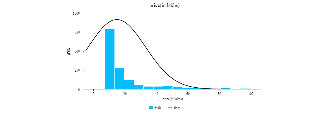
Figure 1. Frequency distribution graph of prices.

It can be observed that the maximum and minimum values of prices are still relatively high, indicating an overall right-skewed distribution in the Figure 1.

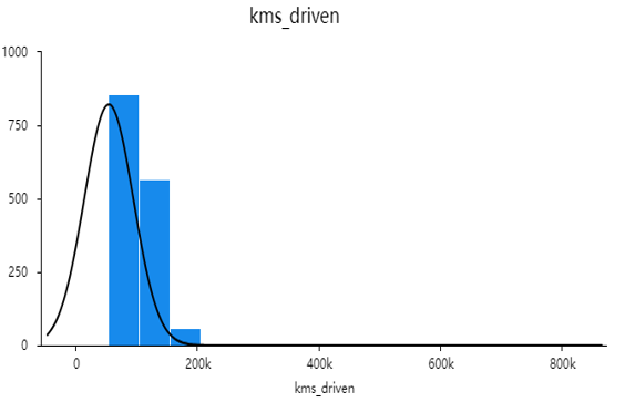
Figure 2. Frequency distribution graph of kms_driven.

The figure 2 in the chart regarding kms_driven for used cars are predominantly high, indicating that second-hand cars or those that have changed hands multiple times tend to have excessive mileage and depreciate in value.

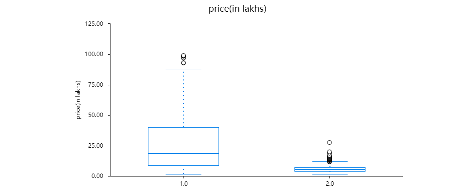
Figure 3. The distribution of Transmission.

A box plot can clearly display the overall distribution of data and, in other scenarios, such as handling outliers, values greater than the upper extreme can be processed (Figure 3).

3.2. Data processing and results

From Figure 4, it can be observed that the Pearson correlation coefficients between price and quantitative factors such as kms_driven, mileage, engine, max_power, and torque are -0.22, 0.05, 0.29, 0.29, and -0.02 respectively. These coefficients indicate that there is a significant negative correlation between kms_driven and price; no significant correlation exists between mileage and price; there is a significant positive correlation between engine size and price; there is also a significant positive correlation between maximum power output (max_power) and price; however, no notable relationship exists between torque and price.

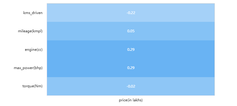
Figure 4. Correlation analysis of each numerical variables with price.

Figure 5. Correlation analysis between numerical variables.

The Figure 5 above shows a study conducted on kms_driven, mileage, engine, max_power, and torque using correlation analysis. The aim was to analyze the relationships between these four variables pairwise by utilizing the Pearson correlation coefficient to indicate the strength of their correlations. Through this analysis, it can be concluded that: The variable kms_driven exhibits significant negative correlations with mileage (kmpl), engine capacity (cc), and maximum power output (bhp) with correlation coefficients of -0.093, -0.102, and -0.102 respectively. These findings suggest a negative association between kms_driven and the aforementioned variables. However, there is no statistically significant correlation observed between kms_driven and torque (Nm), as indicated by a correlation coefficient close to zero.

Table 4. Linear regression analysis results.

In Figure 4, the author eliminates mileage and torque as they are not relevant. Additionally, since the correlation between engine and max_power is 1 (Figure 5), they have the same impact on price. Therefore, one of them is excluded in the multiple linear regression analysis. The author only includes kms_driven and engine in the regression model. From the above table 4, it can be observed that insurance_validity, fuel_type, seats, ownership, transmission, mileage (kmpl), engine (cc), kms_driven, and registration year are taken as independent variables in a linear regression analysis with price (in lakhs) being the dependent variable.

The model formula is as follows: \( price=-1859.053-0.226*insuranc{e_{validity}}+ 2.762*fue{l_{type}}+…+ 0.935*registration year. \)

The model’s coefficient of determination, R-squared, is 0.414, indicating that the variables insurance_validity, fuel_type, seats, ownership, transmission, mileage (kmpl), engine (cc), kms_driven and registration year collectively explain 41.4% of the variation in price (in lakhs). The F-test results show that the model passes the F-test (F=115.804; p=0.000<0.05), suggesting that at least one of the variables insurance_validity, fuel_type, seats, ownership, transmission,mileage(kmpl), engine(cc), kms_driven and registration year has a significant impact on price(in lakhs). Next, this paper will compare their respective p-values; if p-value<0.05 it indicates a significant relationship exists. The positive or negative t-values determine whether there is a positive or negative relationship with price.

After summarizing and analyzing, the author can draw the following conclusions: Fuel_type, seats, engine(cc), and registration_year have a significant positive impact on the price in lakhs. On the other hand, transmission, mileage (kmpl), and kilometers driven have a significant negative impact on the price. However, insurance validity and ownership do not affect the price. The model diagram (Figure 6) illustrates the impact of all analyzed independent variables on the dependent variable. Finally, this study yielded results as shown in Table 5. The dataset demonstrated a Root Mean Squared Error (RMSE) of 13.939 under the multivariate linear regression model.

\( RMSE=\sqrt[]{\sum _{i=1}^{n}\frac{{〖{(\hat{y}〗_{i}}-{y_{i}})^{2}}}{n}} \ \ \ (4) \)

Where \( {\hat{y}_{1}},{\hat{y}_{2}} \) , \( {\hat{y}_{3}} \) ,..., \( {\hat{y}_{n}} \) are predicted values, \( {y_{1}} \) , \( {y_{2}} \) , \( {y_{3}} \) ,..., \( {y_{n}} \) are observed values, and n is the number of observations.

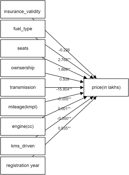
Figure 6. Graph of Multiple Linear Regression Model Results.

Table 5. Calculation results of multiple linear regression model.

4. Conclusion

In this study, the author processed and predicted the final results of second-hand car prices using different regression models, comparing their performance. The data for this study was obtained from the website Kaggle and was processed using programming languages. Irrelevant attributes and data with significant biases were excluded in order to retain 1500 samples. The study utilized linear regression and random forest regression for price prediction, comparing the values and RMSE errors of both models. It was found that the production year of second-hand cars had the greatest impact on prices, but there still remained a relatively large RMSE error. Additionally, it was observed that linear regression and random forest predictions yielded similar results, indicating that there is still considerable room for improvement in developing machine learning pricing models. Future work can build upon this study by utilizing larger datasets to obtain better training data.

In this study, the author utilized various regression models to process and predict the final results of used car prices, comparing their performance. The data for this research was obtained from the website www.kaggle.com and processed using programming languages. Approximately 1500 samples were retained while excluding irrelevant attributes and data with significant biases. The study employed multiple linear regression for price prediction, calculating the model’s R-value and root mean square error. This indicates variables insurance_validity, fuel_type, seats, ownership, transmission, mileage (kmpl), engine (cc), kms_driven and registration year collectively explain 41.4% of the variation in price (in lakhs). The RMSE value of 13.939 is not satisfactory to the author, and a larger dataset may produce better results. The data obtained in this study will aid in predicting used car prices through multiple linear regression analysis.

References

[1]. Monburinon N, et al. 2018 Prediction of prices for used car by using regression models. 2018 5th International Conference on Business and Industrial Research (ICBIR).
[2]. Noor K. and Jan S 2017 Vehicle price prediction system using machine learning techniques. International Journal of Computer Applications, 167(9), 27-31.
[3]. Wang F, Zhang X and Wang Q 2021 Prediction of used car price based on supervised learning algorithm. 2021 International Conference on Networking, Communications and Information Technology (NetCIT).
[4]. Varshitha J, Jahnavi K and Lakshmi C 2022 Prediction of used car prices using artificial neural networks and machine learning. 2022 International Conference on Computer Communication and Informatics (ICCCI).
[5]. Chen Z and Li X 2022 Vehicle price forecasting based on multiple machine learning models. 2022 IEEE Conference on Telecommunications, Optics and Computer Science (TOCS).
[6]. Chen C, Hao L and Xu C 2017 Comparative analysis of used car price evaluation models. AIP Conference Proceedings.
[7]. Krishnan J R and Selvaraj V 2022 Predicting resale car prices using machine learning regression models with Ensemble Techniques. 2ND International Conference on Mathematical Technology and Applications: ICMTA2021.
[8]. Pal N, et al. 2018 How much is my car worth? A methodology for predicting used cars’ prices using random forest. Advances in Intelligent Systems and Computing, 413-422.
[9]. Ponmalar P P and Christinal C A 2022 Review on the pre-owned car price determination using machine learning approaches. 2022 International Conference on Augmented Intelligence and Sustainable Systems (ICAISS).
[10]. Kumar A 2023 Machine learning based solution for asymmetric information in prediction of used car prices. Proceedings in Adaptation, Learning and Optimization, 409-420.
Cite this article
Wang,Y. (2024). Second-hand car price prediction based on multiple linear regression models. Theoretical and Natural Science,39,186-194.
Data availability
The datasets used and/or analyzed during the current study will be available from the authors upon reasonable request.
Disclaimer/Publisher's Note
The statements, opinions and data contained in all publications are solely those of the individual author(s) and contributor(s) and not of EWA Publishing and/or the editor(s). EWA Publishing and/or the editor(s) disclaim responsibility for any injury to people or property resulting from any ideas, methods, instructions or products referred to in the content.
About volume
Volume title: Proceedings of the 2nd International Conference on Mathematical Physics and Computational Simulation
© 2024 by the author(s). Licensee EWA Publishing, Oxford, UK. This article is an open access article distributed under the terms and
conditions of the Creative Commons Attribution (CC BY) license. Authors who
publish this series agree to the following terms:
1. Authors retain copyright and grant the series right of first publication with the work simultaneously licensed under a Creative Commons
Attribution License that allows others to share the work with an acknowledgment of the work's authorship and initial publication in this
series.
2. Authors are able to enter into separate, additional contractual arrangements for the non-exclusive distribution of the series's published
version of the work (e.g., post it to an institutional repository or publish it in a book), with an acknowledgment of its initial
publication in this series.
3. Authors are permitted and encouraged to post their work online (e.g., in institutional repositories or on their website) prior to and
during the submission process, as it can lead to productive exchanges, as well as earlier and greater citation of published work (See
Open access policy for details).