1. Introduction

The acquisition of digital signal audio data is contingent upon the utilization of a pickup device, which inevitably results in the incorporation of a multitude of noise sources. These include airflow sounds, the inherent noise of the pickup device itself, and the noise generated by the original recording source, as well as the reverberation of the recording space. In order to facilitate the identification and processing of these acoustic digital signal data, it is important to exclude noise. The digital signals obtained by picking up sound are typically stored as one-dimensional data at the sampling rate \( Fs \) :

\( X=(x(1),x(2),…,x(n))\ \ \ (1) \)

where \( n \) is the length of the data signal \( X \) , and \( x(t),t=1,2,...,n \) represents the amplitude of the sound waveform sampled every \( \frac{1}{Fs} \) second. And the objective is to obtain another segment of digital signal \( Y \) that is also of length \( n \) but contains less noise. The traditional filter denoising method is to remove some components of the signal by intercepting the Fourier coefficients modulus. However, in reality, noise and pure signals are typically intertwined in the frequency domain. Filtering methods not only results in the loss of useful details but also fails to remove noise in key frequency bands. Other popular denoising methods include the wavelet decomposition and reconstruction method [1] and the wavelet threshold shrinkage method [2]. However, the selection of the wavelet bases and the construction of mother wavelets are not universal in different noise and frequency characteristics. Consequently, it is difficult to devise a method that can be easily applied to audio digital signals.

It is fortunate that the key information in audio data exhibits significant low-rank properties. It is possible to construct a range of models from common audio signals. These include the Damped and Delayed Sinusoidal model (DDS), the Partial Damped and Delayed Sinusoidal model (PDDS), and the Exponentially Damped Sinusoidal model (EDS) [3]. This indicates that some bases can be used to represent real sound vibration patterns and can simulate physical properties well. Furthermore, the Low-Rank Time-Frequency Synthesis model (LRTFS) [4, 5] imposes a low rank on the synthesis coefficients of the data signals, thereby transforming the high-dimensional data into a sparse low-rank representation. The signal reconstructed by combining and transforming these substrates not only has the low-rank property, but also retains the key information. The low-rank structure in high-dimensional data has been validated in numerous research studies, including those employing the Principal Component Analysis (PCA) technique. These studies have demonstrated that a significant proportion of the energy in high-dimensional data is concentrated in a few principal directions, often exceeding 95%.

Due to the low-rank property, denoising effects can be obtained by approximating the original sound with a low-rank structure. In the case of a small amount of data, since the rank of the Hankel matrix of pure signal is twice the number of harmonics[6], low-rank approximation method that directly constructs the Hankel matrix can remove local noise to a large extent[7], like applying low-rank approximation to Magnetic Resonance Spectroscopic Imaging (MRSI) for denoising[8]. However, the time series signal processed is usually a large dataset, and the Hankel matrix constructed directly from \( X \) contains \( {n^{2}} \) components. The most common audio files in WAV format have a sample rate of up to 44,100 times per second, which presents a significant challenge for data storage and matrix operations.

This paper proposes the windowed singular value decomposition (WSVD) of frequency division and employs low-rank approximation for fast singular value decomposition. The algorithm decomposes the signal into different frequency bands and adds a window to segment the digital signal. Furthermore, Lanczos bidiagonalization [9] iterations are employed in the key singular value decomposition step, thereby enhancing the efficiency of the algorithm. An additional denoising technique is employed in the edges of windows to ensure the signal's consistency and coherence. Therefore, this paper is organized as follows. Chapter 2 describes the algorithm in detail. Chapter 3 presents numerical simulation and experimental results, and analyses the denoising effectiveness, time performance, and robustness of the results to different judgment levels using different evaluation Indicators. Chapter 4 further discusses the feasibility of low-rank approximation and the role of frequency division. Finally, Chapter 5 presents the conclusion.

2. Proposed Denoising Method based on Low-Rank Approximation

2.1. Foundations of the Low-Rank Models

Low-rank approximation methods are based on the low-rank characteristics observed in audio digital signals. In particular, audio exhibits two aspects of low-rank local characteristics: a stable resonance due to a relatively fixed pitch, and a similar formant due to the same timbre and feature information.

The measured data is denoted as \( X=Y+Ε \) , where \( Ε={(ϵ(t))_{t=1,2,…,n}} \) represents the component of noise, which is typically modeled as additive Gaussian white noise (AGWN) in simulation experiments. Contemporary signal detection and classification methodologies are capable of accurately constructing noise models derived from authentic sources. These include the Gaussian Mixture Model (GMM) [10, 11] and the α Stable Distribution Noise Model [12], as well as the Middleton Class A noise model (MCA) [13], which is a more challenging endeavor. Noise exhibits instability in both the temporal and spatial domains. However, the noise occupies a relatively small amount of energy, with the majority of the remaining energy concentrated in the key information. Consequently, a low-rank approximation can be employed to extract the subspace in which the main energy is collected.

The model of a uniformly sampled damped sinusoidal signal can be generally expressed as follows:

\( x(t)=s(t)+ϵ(t) \)

\( =\sum _{k=1}^{N}{A_{k}}{e^{i{Φ_{k}}}}{e^{(-{α_{k}}+i2π{f_{k}})t}}+ϵ(t)\ \ \ (2) \)

where \( x(t) \) is the measured data, \( s(t) \) and \( ϵ(t) \) denote the pure signal and noise, \( s(t) \) consists of damped sinusoidal signal bases, \( N \) is the total number of harmonics, and \( {A_{k}} \) , \( {α_{k}} \) , \( {f_{k}} \) , and \( {Φ_{k}} \) \( (k=1,2,...,N) \) denote amplitude intensity, damping rate, frequency, and initial phase of the \( {k^{th}} \) harmonic component, respectively[6].

2.2. Constructing Hankel Matrices for Low-Rank Representations

In order to facilitate the study of time-series signal data \( X \) in long strips, the signal can usually be constructed in the form of a Hankel matrix:

\( H=[\begin{matrix}x(1) & x(2) & ⋯ & x(K) \\ x(2) & x(3) & ⋯ & x(K+1) \\ ⋮ & ⋮ & ⋱ & ⋮ \\ x(n-K+1) & x(n-K+2) & ⋯ & x(n) \\ \end{matrix}]\ \ \ (3) \)

In general, to better analyze the correlation, \( K=⌊\frac{n+1}{2}⌋ \) can be chosen. In particular, when \( n \) is odd, \( H \) is a symmetric matrix. The DSS model also shows that time series signals have strong linear predictability over time, i.e.

\( x(m)=\sum _{l=1}^{M}{β_{l}}x(m-l\cdot Δt)\ \ \ (4) \)

where \( M \) is the predicted order, \( {β_{l}} \) is the predicted coefficient, and \( Δt \) is the sample interval. Due to the strong linear predictability, the \( {m^{th}} \) component of the signal \( X \) can also be estimated by the \( M \) terms preceding it. At this juncture, the Hankel matrix constructed has a rank of \( M \) [8].

A proof of the low rank of the undamped and delayed sinusoidal model signal will be given, and it will be verified again with simulation in Section 4. For brevity of the proof, it is assumed that the waveform is a superposition of sinusoids, and that the waveform of signal can be represented as:

\( x(t)=\sum _{k=1}^{N}{A_{k}}sin{({f_{k}}t)}\ \ \ (5) \)

Now \( X \) represents a noiseless signal, and the damping and delay effects are not considered in this case. Assuming that the audio signal is sampled at time intervals of \( Δt \) , starting from \( {t_{1}} \) , the signal can be expressed as \( x(t)=\sum _{k=1}^{N}{A_{k}}sin{({f_{k}}({t_{1}}+(t-1)Δt))}, t=1,2,…,n \) and the Hankel matrix can be defined as follows:

\( H=[\begin{matrix}x(1) & x(2) & ⋯ & x(q) \\ x(2) & x(3) & ⋯ & x(q+1) \\ ⋮ & ⋮ & ⋱ & ⋮ \\ x(p) & x(p+1) & ⋯ & x(p+q-1) \\ \end{matrix}]\ \ \ (6) \)

where \( p=⌈\frac{n+1}{2}⌉,q=⌊\frac{n+1}{2}⌋ \) . It can be demonstrated that the rank of the matrix \( H \) is at most \( 2N \) .

Lemma1.

Assuming that \( {H_{k}}={(h_{ij}^{(k)})_{p×q}}∈{R^{p×q}} \) , where \( h_{ij}^{(k)}=sin{({f_{k}}({t_{1}}+(i+j-2)Δt))} \) , then \( rank({H_{k}})≤2 \) can be obtained.

Proof:

\( ∀1≤i≤p,1≤j≤q \) , the following equation can be derived:

\( h_{ij}^{(k)}=sin{({f_{k}}{t_{1}}+{f_{k}}(i+j-2)Δt)} \)

\( =sin{({f_{k}}({t_{1}}-2Δt)+{f_{k}}Δt\cdot i)}cos{({f_{k}}Δt\cdot j)}+sin{({f_{k}}Δt\cdot j)}cos{({f_{k}}({t_{1}}-2Δt)+{f_{k}}Δt\cdot i)} \)

\( =ϕ_{k}^{(1)}(i){ψ_{k}^{(1)}(j)}+ϕ_{k}^{(2)}(j)ψ_{k}^{(2)}(i) \)

where \( ϕ_{k}^{(1)},ϕ_{k}^{(2)}{,ψ_{k}^{(1)}},ψ_{k}^{(2)} \) are functions with parameters \( {f_{k}},{t_{1}},Δt \) .

Therefore,

\( {H_{k}}={(h_{ij}^{(k)})_{p×q}}={[\begin{matrix}ϕ_{k}^{(1)}(1) & ψ_{k}^{(2)}(1) \\ ⋮ & ⋮ \\ ϕ_{k}^{(1)}(i) & ψ_{k}^{(2)}(i) \\ ⋮ & ⋮ \\ ϕ_{k}^{(1)}(p) & ψ_{k}^{(2)}(p) \\ \end{matrix}]_{p×2 }}{[\begin{matrix}ψ_{k}^{(1)}(1) & ⋯ & ψ_{k}^{(1)}(j) & ⋯ & ψ_{k}^{(1)}(q) \\ ϕ_{k}^{(2)}(1) & ⋯ & ϕ_{k}^{(2)}(j) & ⋯ & ϕ_{k}^{(2)}(q) \\ \end{matrix}]_{2×q}}={P_{1}}{P_{2}} \)

Since \( {P_{1}} \) has only two columns and \( {P_{2}} \) has only two rows, the rank of \( {P_{1}} \) and \( {P_{2}} \) satisfy:

\( rank({P_{1}})≤2,rank({P_{2}})≤2 \)

So

\( rank({H_{k}})=rank({P_{1}}{P_{2}})≤min{\lbrace rank({P_{1}}),rank({P_{2}})\rbrace }=2\ \ \ \)

Theorem1.

Let \( X \) be a signal acquired at a constant sampling rate that is consistent with an undamped and delayed sinusoidal model, whose highest order of resonance is \( N \) . Then, the rank of the Hankel matrix \( H \) constructed by the signal is at most \( 2N \) .

Proof:

Assuming that \( H={({h_{ij}})_{p×q}} \) is of the form as (6), then in accordance with equation (5) and Lemma 1, the Hankel matrix can be expressed as a linear combination of specific matrices.:

\( H={({h_{ij}})_{p×q}}={(\sum _{k=1}^{N}{A_{k}}h_{ij}^{(k)})_{p×q}}=\sum _{k=1}^{N}{A_{k}}{(h_{ij}^{(k)})_{p×q}}=\sum _{k=1}^{N}{A_{k}}{H_{k}} \)

Since \( {A_{k}} \) is an invariant coefficient, \( rank({A_{k}}{H_{k}})=rank({H_{k}}) \) .

So, the rank of the constructed Hankel matrix can be obtained:

\( rank(H)=rank(\sum _{k=1}^{N}{A_{k}}{H_{k}})=rank(\sum _{k=1}^{N}({A_{k}}{H_{k}})) \)

\( ≤\sum _{k=1}^{N}rank({A_{k}}{H_{k}})≤2N\ \ \ \)

2.3. Low-rank Approximation Methods

It is assumed that the Hankel matrix \( H∈{R^{p×q}} \) is formed from the audio signal, with \( p ≥ q \) . The denoising effect is then achieved by applying low-rank approximation. The objective is to obtain an approximate optimal Hankel matrix \( {H^{*}} \) , for which the corresponding regularization problem is:

\( \underset{{H^{*}}}{min}{{‖{H^{*}}-H‖_{F}}} s.t. rank({H^{*}})≤{L_{1}}\ \ \ (7) \)

The solution to this problem is the hard threshold algorithm for singular value decomposition (SVD). The initial step is to decompose the matrix \( H \) into the following form:

\( H=US{V^{T}}={[{u_{1}}{u_{2}}…{u_{p}}]_{p×p}}[\overline{\begin{matrix}{σ_{1}} & & & \\ & {σ_{2}} & & \\ & & ⋱ & \\ & & & {σ_{q}} \\ \end{matrix}} \\ 0]{[\begin{matrix}v_{1}^{T} \\ v_{2}^{T} \\ ⋮ \\ v_{q}^{T} \\ \end{matrix}]_{q×q}} \)

\( ={σ_{1}}{u_{1}}v_{1}^{T}+{σ_{2}}{u_{2}}v_{2}^{T}+…+{σ_{q}}{u_{q}}v_{q}^{T}\ \ \ (8) \)

where \( U \) , \( V \) are orthogonal matrices and \( S \) is a diagonal matrix consisting of singular values \( {σ_{k}}(1≤k≤q) \) arranged from largest to smallest. \( {u_{i}},{v_{j}}(1≤i≤p, 1≤j≤q \) ) are left and right singular vectors respectively. Now the first \( {L_{1}} \) singular values are selected and the rest of the singular values are set to \( 0 \) to obtain a new diagonal matrix \( {S^{*}} \) , and the matrix is reconstructed as follows:

\( {H^{*}}=U{S^{*}}{V^{T}}\ \ \ (9) \)

Then the optimal approximation for problem (7) is obtained. And

\( {H^{*}}={σ_{1}}{u_{1}}v_{1}^{T}+{σ_{2}}{u_{2}}v_{2}^{T}+…+{σ_{{L_{1}}}}{u_{{L_{1}}}}v_{{L_{1}}}^{T}={(h_{ij}^{*})_{p×q}}\ \ \ (10) \)

Subsequently, the signals are extracted from \( {H^{*}} \) by merging the transpose of the first column of \( {H^{*}} \) and the last row with the first component removed, and then recomposing it into a new vector \( Y \) , where each element of \( Y \) is

\( y(t)=\begin{cases} h_{t1}^{*} , 1≤t≤p \\ h_{p,t-p+1}^{*} , p+1≤t≤n\end{cases}\ \ \ (11) \)

Thus, the optimal solution for the low-rank approximation vector is obtained. The space and time complexity of the computation is now considered. According to the traditional method, the following theorem can be demonstrated:

Theorem2.

A complete SVD of a matrix \( H \) is computationally equivalent to computing the eigenvalues and eigenvectors of the matrices \( {H^{T}}H \) and \( {HH^{T}} \) .

Proof:

Noting that \( {H^{T}}H \) and \( {HH^{T}} \) are all semi-positive definite symmetric matrices, they are all diagonalizable and have non-negative eigenvalues, so

\( {H^{T}}H={(US{V^{T}})^{T}}(US{V^{T}}) \)

\( =(V{S^{T}}{U^{T}})(US{V^{T}}) \)

\( =V{S^{T}}{U^{T}}US{V^{T}} \)

\( =V{S^{T}}S{V^{T}} \)

Let \( L={S^{T}}S∈{R^{q×q}} \) as a diagonal matrix as well, the components of which are \( {λ_{k}}=σ_{k}^{2}(1≤k≤q) \) , then

\( {H^{T}}H=VL{V^{T}} \)

\( {H^{T}}HV=VL \)

which satisfies \( ∀k∈\lbrace 1,2,…,q\rbrace \) ,

\( {H^{T}}H{v_{k}}={λ_{k}}{v_{k}} \)

Therefore, the eigenvectors of \( {H^{T}}H \) are the right singular vectors, and squaring their eigenvalues gives the singular values \( {σ_{k}}=\sqrt[]{{λ_{k}}} \) .

Similarly, there exists \( \widetilde{L}∈{R^{p×p}} \) such that the eigenvalues and eigenvectors satisfy \( H{H^{T}}U=U\widetilde{L} \) , which is fulfilled by \( ∀k∈\lbrace 1,2,…,p\rbrace \) ,

\( H{H^{T}}{u_{k}}={λ_{k}}{u_{k}} \)

Therefore, the eigenvectors of \( {HH^{T}} \) are the left singular vectors. □

According to Theorem 2, the computational complexity should be extremely high when \( n \) is large. The size of the Hankel matrix generated by a signal \( X \) of length \( n \) is about \( {n^{2}}/4 \) . On the one hand, this size is enormous. For example, a one-minute audio signal (which is usually much longer in practice) with a sampling rate of 44,100 has \( {(44100×60)^{2}}≈7×{10^{12}} \) components in the constructed matrix, which would require more than the limit of memory in double precision data, not to mention transformation and transition matrices. On the other hand, the computational complexity is high, e.g. the Golub-Reinsch SVD algorithm and the R-SVD algorithm require at least \( 4{pq^{2}}-4{q^{3}}/3 \) and \( 2{pq^{2}}+2{q^{3}} \) steps respectively.

Noticing that only the first \( k \) singular values and singular vectors are needed, Lanczos bidiagonalization can be used to compute SVD, which exploits the principle that singular values of a matrix are invariant in orthogonal transformations. The algorithm is as follows:

Firstly, turn \( H \) into an upper bidiagonal form by orthogonal transformations:

\( {\widetilde{U}^{T}}H\widetilde{V}=[\overline{\begin{matrix} {α_{1}} & {β_{1}} & & & \\ & {α_{2}} & {β_{2}} & & \\ & & ⋱ & ⋱ & \\ & & & {α_{q-1}} & {β_{q-1}} \\ & & & & {α_{q}} \\ \end{matrix}} \\ 0]\ \ \ (12) \)

In practice, instead of applying Householder transform for diagonalization, which produces dense submatrices in the middle, the Golub-Kahan upper diagonalization is applied to directly solve for \( {U_{k}}∈{R^{p×k}},{B_{k}}∈{R^{k×k}},{V_{k}}∈{R^{q×k}} \) such that

\( {H^{*}}={U_{k}}{B_{k}}V_{k}^{T}={[\widetilde{{u_{1}}}\widetilde{{u_{2}}}…\widetilde{{u_{k}}}]_{p×k}}[\begin{matrix}{α_{1}} & {β_{1}} & & & \\ & {α_{2}} & {β_{2}} & & \\ & & ⋱ & ⋱ & \\ & & & {α_{k-1}} & {β_{k-1}} \\ & & & & {α_{k}} \\ \end{matrix}]{[\begin{matrix}\widetilde{v_{1}^{T}} \\ \widetilde{v_{2}^{T}} \\ ⋮ \\ \widetilde{v_{k}^{T}} \\ \end{matrix}]_{k×q}}\ \ \ (13) \)

This algorithm employs the Lanczos bidiagonalization to directly generate the bidiagonal entries, circumventing the intermediate material of the conventional Householder bidiagonalization. The process is described as follows:

ALGORITHM 1: Golub-Kahan Bidiagonalization

Initialization: The first column of \( {V_{k}} \) , designated \( {v_{c}} \) , is to be formed by selecting a set of normal distributed random numbers.

\( k=0,{p_{0}}={v_{c}},{β_{0}}=‖{p_{0}}‖,{u_{0}}=0 \)

while \( {β_{k}}≠0 \) do

\( {v_{k+1}}={p_{k}}/{β_{k}} \)

\( k=k+1 \)

\( {r_{k}}=H{v_{k}}-{β_{k-1}}{u_{k-1}} \)

\( {α_{k}}=‖{r_{k}}‖ \)

\( {u_{k}}={r_{k}}/{α_{k}} \)

\( {p_{k}}={H^{T}}{u_{k}}-{α_{k}}{v_{k}} \)

\( {β_{k}}=‖{p_{k}}‖ \)

end

After \( k \) iterations, this algorithm will eventually yield \( {U_{k}}=[{u_{1}}|…|{u_{k}}],{V_{k}}=[{u_{1}}|…|{u_{k}}] \) and a upper bidiagonal matrix \( {B_{k}} \) , which satisfies

\( H{V_{k}}={U_{k}}{B_{k}} \)

\( {H^{T}}{U_{k}}={V_{k}}B_{k}^{T}+{p_{k}}e_{k}^{T}\ \ \ (14) \)

where \( {e_{k}} \) denotes the \( {k^{th}} \) column of the identity matrix. According to the Lanczos convergence theory of symmetric matrices, good approximations to large singular values of \( H \) emerge at an early stage. Subsequently, compute the SVD of \( {B_{k}} \) :

\( F_{k}^{T}{B_{K}}{G_{k}}={S_{k}}=diag({s_{1}},…,{s_{k}})\ \ \ (15) \)

Then final result is obtained:

\( {Y_{k}}={U_{k}}{F_{k}}=[{y_{1}},…,{y_{k}}] \)

\( {Z_{k}}={V_{k}}{G_{k}}=[{z_{1}},…,{z_{k}}]\ \ \ (16) \)

In accordance with the Ritz Approximations theorem, by setting \( k={L_{1}} \) , the first \( k \) largest singular values \( {σ_{i}} \) of \( H \) are approximated as \( {s_{i}}(1≤i≤k) \) , and the corresponding first \( k \) columns of the singular vector matrices \( U \) and \( V \) are approximated as \( {Y_{k}} \) and \( {Z_{k}} \) . The procedure outlined above describes the method for computing the first \( k \) largest singular values and the first \( k \) singular vectors using Lanczos bidiagonalization.

In order to guarantee the precision of the outcomes and to prevent the algorithm from skipping over larger singular values and converging on smaller ones, a loop was set up to restart Lanczos bidiagonalization for \( k+1 \) until the first \( k \) singular values had converged. The workload of applying the Lanczos bidiagonalization method is \( O({k^{3}}) \) , which is considerably less than the original \( O({p^{2}}q) \) .

2.4. Rank Determination

One simple method is to set \( {L_{1}} \) based on the number of harmonics. However, in practice, it is preferable to select a larger \( {L_{1}} \) in consideration of the impact of amplitude, damping and delay. Another approach is to determine \( {L_{1}} \) using autoregressive models[8, 14], which let \( \underset{\hat{L}}{min}{|AIC(\hat{L})-AIC(\hat{L}+1)|} \) to be the optimal choice of \( {L_{1}} \) , where \( AIC(\hat{L})=Mlog{e(\hat{L})}+2\hat{L} \) . In order to deal with various noises, an empirical rank can also be selected for approximation. In the algorithms, the ratio of singular values is specified as a parameter, which reflects the rank proportion selected.

2.5. Core Improvement Methodology

To accommodate noises with different frequency characteristics, the sounds in each band of \( X \) are separated over a period of time with an interval of \( n \) before subsequent processing.

ALGORITHM 2: Modulus Classification

Initialization: \( n \) is the length of \( X \) , Fs is the sampling rate, and set \( f_{i}^{(1)},f_{i}^{(2)} \) as the upper and lower bounds of each frequency band,

\( {F_{X}}=fftshift(fft(\frac{X}{n})) \)

\( f=abs(linspace(-\frac{fs}{2},\frac{fs}{2}-1,n)) \)

while \( 0≤f_{i}^{(1)} \lt f_{i}^{(2)}≤2.2×{10^{4}} \) do

\( {X_{{f_{i}}}}={F_{X}}⊙(f_{i}^{(1)} \lt f \lt f_{i}^{(2)}) \) i.e. set modulus of the other bands to 0

\( {X_{i}}=Real(ifft(ifftshift({X_{{f_{i}}}}))) \) i.e. reconstruct the signal

end while

To further increase the computational speed and make use of the locally low-rank nature of the audio, a low-rank approximation method is applied in a small window of fixed length per segment.

ALGORITHM 3: Windowed Singular Value Decomposition (WSVD)

Initialization: For each segment \( {X_{i}} \) , choose \( {w_{i}} \) as the length of the window and \( {L_{i}} \) as the order for the approximation.

for \( k=1,2,…,⌊\frac{n}{{w_{i}}}⌋ \) loop

\( H←{X_{i}}(k{w_{i}}-{w_{i}}+1:k{w_{i}}) \)

\( {B_{k}},{Y_{k}},{Z_{K}}←compute SVD of order k of H by Lanszos bidiagonalization \)

\( {H^{*}}←{Y_{k}}{B_{k}}Z_{k}^{T} \)

\( {Y_{i}}(k{w_{i}}-{w_{i}}+1:k{w_{i}})←{H^{*}} \)

end loop

Remark: If the window length \( {w_{i}} \) does not divide \( n \) integrally, extend the last window to the end.

Ultimately, the reconstruction \( Y={Σ_{i}}{Y_{i}} \) is the final result. The overall process of denoising algorithm with WSVD of frequency division is as follows, the first step is to select \( n \) as length of each audio segment and select the nodes for dividing the frequency bands, then apply Algorithm 1 to obtain the divided signal; the second step is to determine the length of the window for each band and select the ratio of the singular values, and apply Algorithm 2 to obtain the denoised signal; and the last step is to reconstruct the final signal by summing the resulting signals.

2.6. Smoothness Techniques

Because audio often has different characteristics over time, the continuity of the denoising can be affected, especially when a high level in one window is followed by a low level in another. Such a situation can lead to unevenness around the boundary between the two windows, such as the resulting “spikes” in the waveform.

One possible approach is to apply a mean filter at each junction, which entails a minimal additional computational expense. An alternative is to perform a two-window interleaved WSVD of frequency division denoising of the original X and replace it with another segment near the window edges. Applying this smoothing technique after each denoising step effectively avoids the appearance of noise, even though the probability of a large difference in nature between the two windows is very small.

3. Results and Analysis

3.1. Evaluation Indicators

3.1.1. Signal-to-Noise Ratio (SNR).

\( SNR=10{log_{10}}{\frac{‖{X_{0}}‖}{‖Y-{X_{0}}‖}}\ \ \ (17) \)

Where \( {X_{0}} \) and \( Y \) represent the original useful signal and the denoised signal respectively. SNR is the ratio of the power of the original signal to the power of the error signal. In the simulation results, higher SNR indicates better denoising effects.

3.1.2. Normalized Correlation Coefficient (NCC).

\( NCC=\frac{\sum _{k=1}^{n}x(k)y(k)}{\sqrt[]{（\sum _{k=1}^{n}{x^{2}}(k)）(\sum _{k=1}^{n}{y^{2}}(k))}}\ \ \ (18) \)

\( x(k),y(k)(1≤k≤n) \) denote the original and denoised signals, respectively. NCC reflects the overall similarity before and after denoising, independent of the details of the waveform oscillatory variations. The closer NCC is to \( 1 \) , the more similar the two signals are, and the less shifted and uncorrelated they are.

3.1.3. Root-mean-square Error (RMSE).

\( RMSE=\sqrt[]{\frac{\sum _{k=1}^{n}{({x_{0}}(k)-y(k))^{2}}}{n}}\ \ \ (19) \)

\( {x_{0}}(k),y(k)(1≤k≤n) \) denote the pure and denoised signals, respectively. RMSE reflects the difference between the pure signal and the signal after denoising, and a smaller RMSE reflects better denoising effects.

3.1.4. Noise Reduction Ratio (NRR).

\( NRR=10{log_{10}}{(\frac{σ_{X}^{2}}{σ_{Y}^{2}})}\ \ \ (20) \)

where \( {σ_{x}} \) and \( {σ_{Y}} \) are the standard deviation of the detected signal and denoised signal, respectively. NRR is used to evaluate the denoising effect without using the pure signal as a reference.

3.1.5. Time Ratio (TR).

\( TR=\frac{{T_{measure}}}{{T_{0}}}\ \ \ (21) \)

where \( {T_{measure}} \) is the time for computation and \( {T_{0}} \) is defined as the time required to compute \( {10^{10}} \) additions. All the numerical simulations in this paper are implemented by MATLAB R2024a in a PC with 16.0 GB RAM and 4 CPUs of 3.10 GHz. All measured times will be divided by \( {T_{0}} \) for reference.

3.2. Simulation and Experiment

In simulations, an analogue signal or dry voice is selected as the pure signal \( {X_{0}} \) , and noise \( Ε \) is introduced into different models to obtain \( X \) . Algorithms are then applied to obtain \( Y \) . In experiments, \( X \) is directly detected, and a comparison is made with denoised \( Y \) .

3.2.1. Evaluation of Denoising Performance. For Simulation 1, a guitar audio signal and a normally distributed random signal are selected as AGWN to compare the effect of frequency-divided WSVD with wavelet denoising and Gaussian filter denoising.

Table 1. Comparison of Denoising Effect

In this simulation, 1000Hz and 3500Hz are selected as nodes according to the original spectrum, the window sizes are set to 150, 100 and 100 respectively, and the selected singular value ratios are set to 0.08, 0.12 and 0.01. According to Table 1, the result shows that WSVD of frequency division can denoise effectively while maintaining the waveform similarity and the trend of change, and also show that the WSVD of frequency division has a better performance compared with other denoising methods.

For Simulation 2, a segment of vocal audio signal is selected and AWGN is added to analyze the effect of the choice of window width and singular value ratio on the results. In this case, the frequency division operation is not performed, and instead, the effect of the window length and the choice of the singular value ratio are considered. As can be seen from Table 2, it is important to choose the correct window length and the appropriate singular values ratio. If the window size is too large, not only will the computation time be longer, but the denoising effect may also be worse because of the weakening of the local low-rank property. If the window size is insufficient, the regularity of the signal may not be adequately captured, resulting in a poor separation from the subspace of noise. Likewise, if the number of singular values is excessive, the noise components will be entrained, and if the number is insufficient, critical information will be lost.

Table 2. Comparison of Results for Window Width and Choice of Singular Values Ratio

3.2.2. Evaluation of Denoising Efficiency. In Experiment 1, musical instrument audio signals of different time lengths with a sampling rate of 44100 are selected to compare the temporal performance and results of full SVD denoising, full WSVD denoising, and WSVD denoising with the application of Lanczos bidiagonalization (as shown in Table 3).

Table 3. Comparison of TR for Audio of Different Time Lengths

The first row of the Table 3 shows the duration of the processed audio, with a window of length 1000 for the signal and the ratio of the selected singular values set to 0.1. Full SVD denoising terminates the computation early for audio with a duration of 1s or more, as the memory required to construct the Hankel matrix exceeds the limit. On the contrary, WSVD effectively avoids the problem of memory shortage. The temporal performance of applying Lanczos bidiagonalization WSVD for denoising is significantly better than that of full WSVD denoising. The superiority of Lanczos bidiagonalization becomes even more obvious if a longer window width is set and smaller singular values ratio are chosen.

3.2.3. Evaluation of robustness. Simulation 3 shows the denoising effect on special audios.

(a) (b)

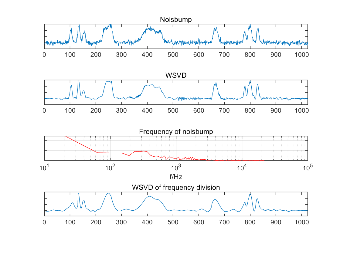
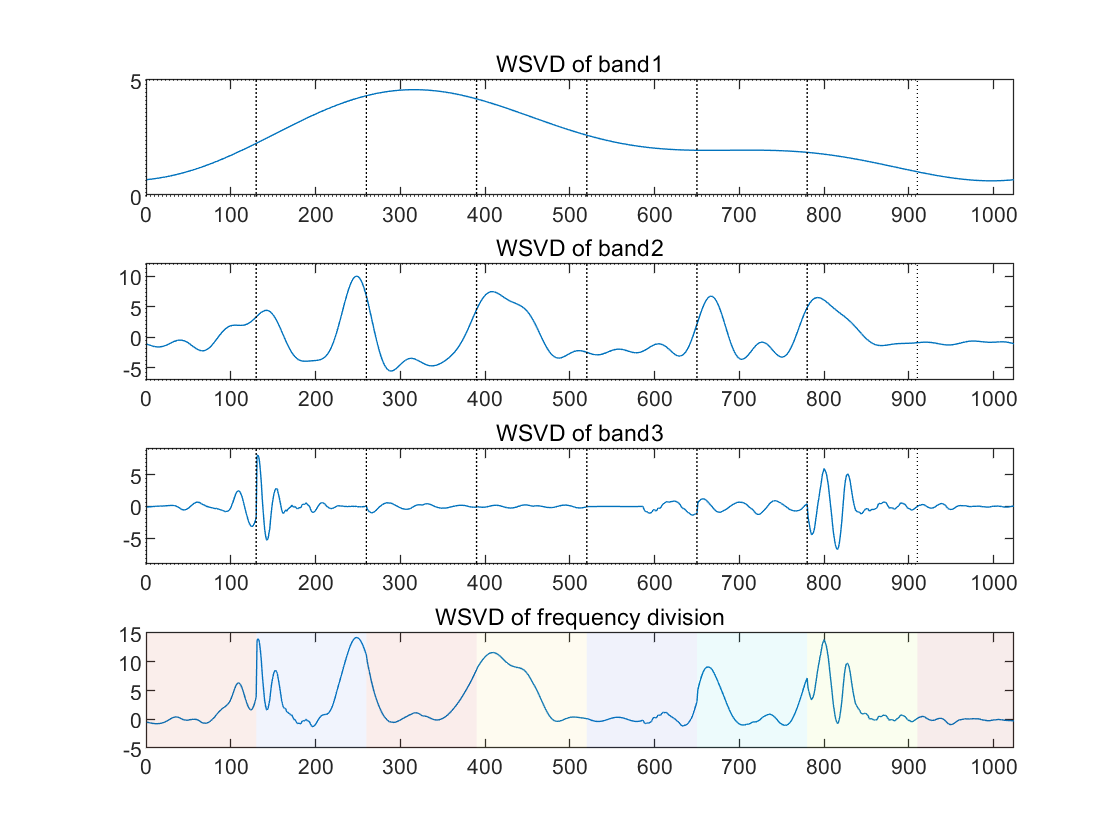
Figure 1. Denoising the “Noisbump” Signal Using WSVD (a. The waveforms of the signal with noise, the waveform of the denoised signal directly using WSVD, the spectrum of the signal with noise and the waveform of the denoised signal using WSVD of frequency division based on the spectrum (from top to bottom); b. The waveforms of the three frequency bands after denoising with 100 Hz and 900 Hz as the dividing points, and the waveform of the reconstructed signal, where the vertical lines in the graph represent the boundaries of the windows)

The simulation denoise the ‘Noisbump’ signal using WSVD (as shown in Figure 1). Typically, the vibrational form of audio signals is not so chaotic, as it resembles noise. However, in order to assess the resilience of the algorithm, WSVD and frequency-divided WSVD were tested. The results demonstrate that WSVD produces suboptimal outcomes in certain windows where noise energy constitutes a significant portion. However, the denoising efficacy of frequency-divided WSVD is considerably superior (a. as shown in the second panel and the last panel of Figure 1.a). In this simulation, WSVD was employed on three signal bands with 100Hz and 900Hz as the frequency division node and the ratio of singular values was selected as 0.4, 0.2 and 0.03, respectively. The final reconstructed signals were able to extract signal features of different frequency bands. In this instance, the window width of each band was set to 130. In a practical application, a smaller window could be employed, with a greater number of singular values selected in the frequency bands where the features are concentrated.

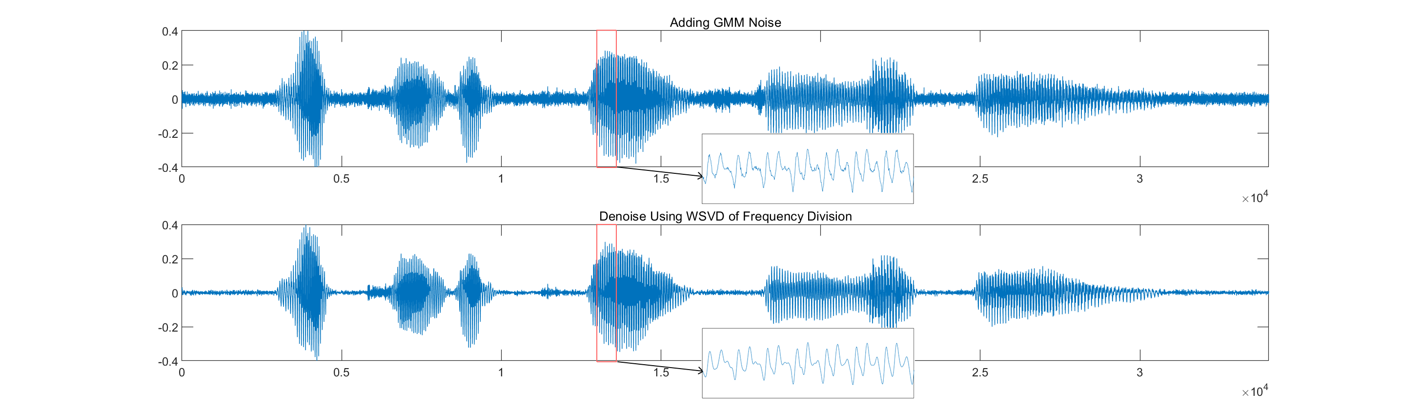
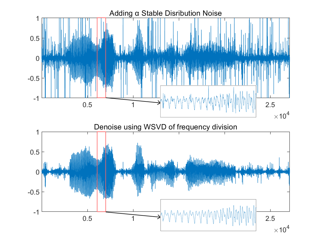
For Simulation 4, the speech signals are selected and non-additive noise (GMM noise, α-stable distribution noise, and MCA noise) is added to test the applicability of WSVD.

(a)

(b) (c)

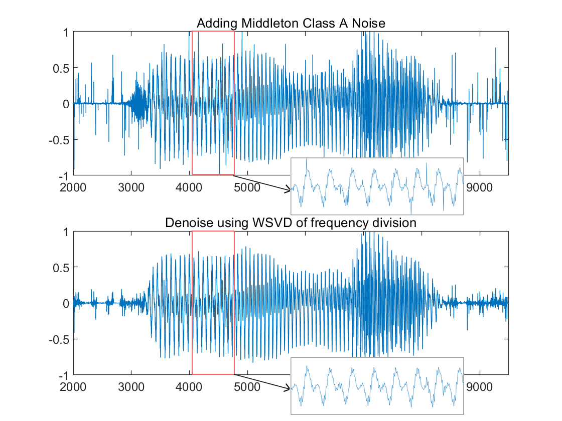
Figure 2. Denoising Results on Signals with Non-additive Noise with Frequency-divided WSVD (a. Adding GMM noise; b. Adding strong α-stable distribution noise; c. Adding MCA noise.)

The WSVD of frequency division can be adapted to different types of noise. In the case of GMM noise, where the noise energy is concentrated at high frequencies, a smaller singular values ratio is chosen in the high frequency band. The noise is effectively attenuated whilst the key signal is retained intact (as shown in Figure 2.a). Even though the α-stable distribution noise and MCA noise with transient impacts are difficult to deal with, the noise occupies a subspace with fewer dimensions and is almost uncorrelated with the subspace in which the signal is located. Therefore, a large portion of the noise can be removed by low-rank approximation (as shown in Figure 2.b, 2.c). The results show that the algorithm is effective for non-additive noise, but in any case, the WSVD works best only when there is a small amount of AWGN.

4. Discussion

In order to ascertain the potential of low-rank approximation in a variety of contexts, this paper conducts an experiment using Monte Carlo cast points to generate random signals.

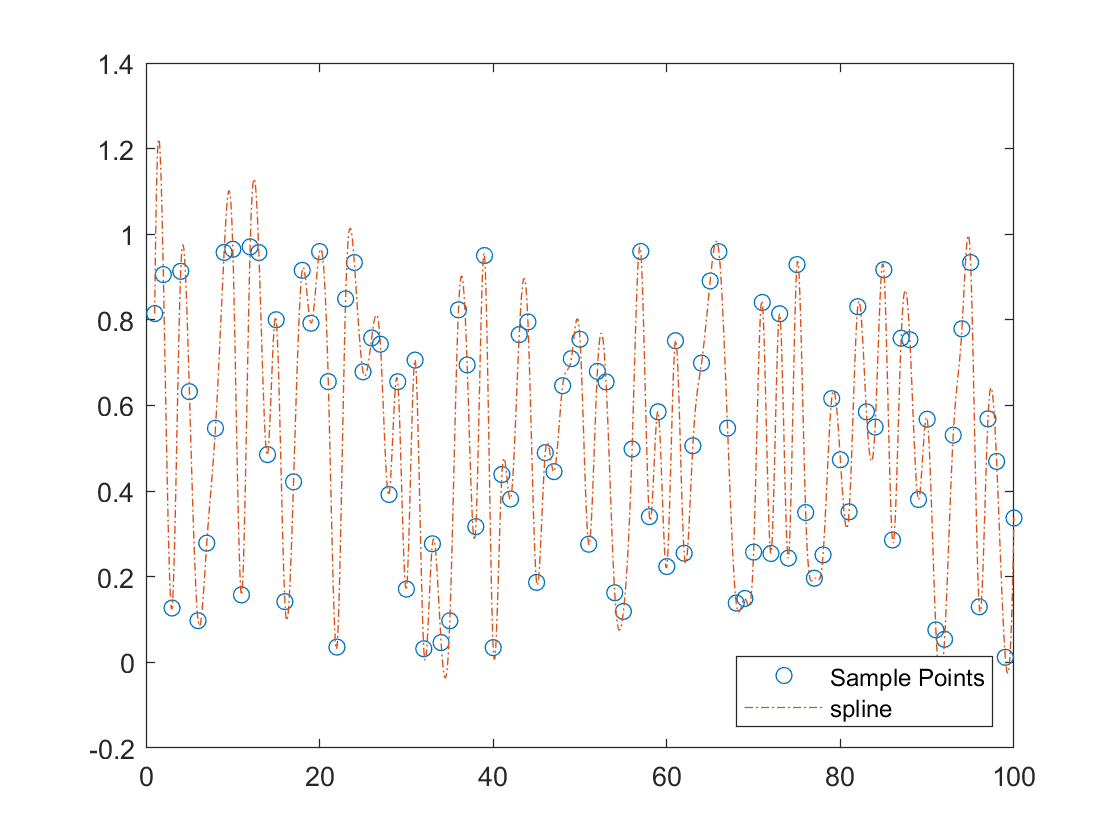
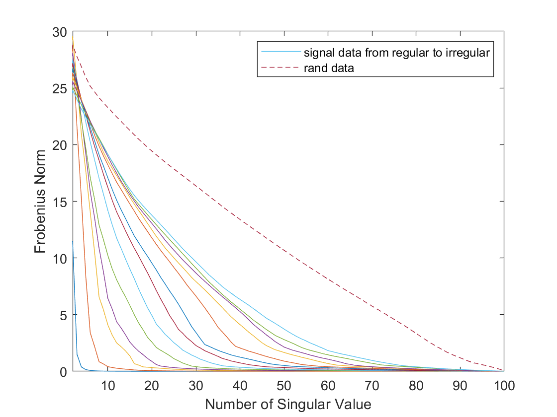
(a) (b)

Figure 3. Results on random signals (a. Cubic spline interpolated digital signal generated from equally spaced random samples. b. Relationship between the number of singular values selected and the Frobenius norm of error according to the signal, at a sampling interval d, with d increasing from the smallest to the largest. The uppermost curve represents the outcome for completely random noise.)

This cubic spline interpolation produces a signal that mimics the vibrational pattern of real audio and retains a good degree of smoothness (as shown in Figure3.a). The obtained signal sample rates range from large to small, representing regular to irregular signals. It can be demonstrated that the selected singular value ratio has a significant impact on the reconstruction quality of the Hankel matrix. According to Figure3.b, for vibrationally regular signals, only a very small number of singular values and singular vectors are needed to reconstruct them. The Frobenius norm of the error of the reconstructed signal is almost linearly related to that of a purely noisy signal. Given that low-rank signals exhibit a high degree of concentration in a limited number of principal directions, it can be reasonably assumed that the scope for optimization in denoising is considerable, provided that the signal is not entirely noise.

For Simulation 5, The Hankel matrix data constructed from the pure sine wave analogue signals are analyzed, which is sampled at 10 intervals for \( {10^{4}} \) data points (as shown in Figure4.a). The harmonic amplitudes are corresponding to the harmonics of the piano sound measured (as shown in Figure4.b). The harmonic components increase from the top to the bottom of the graph. Results show that the rank of the Hankel matrix is not affected by machine error although the harmonics of the simulated sinusoidal signal gradually increase. Each time the harmonics increase by 1, the Hankel matrix constructed from the signal increases by 2. In the full rank case of the Hankel matrix with \( rank=500 \) , the effective information of a signal with 10th harmonics requires only 20 dimensions to reconstruct it completely. Then envelope of the volume was added to the original waveform, modelling the amplification and attenuation of the signal sampled at 10 intervals for \( {5×10^{3}} \) data points (as shown Figure 4.c). At this point, the frequency is concentrated in the region of the formant (as shown in Figure4.d). The full rank case of the Hankel matrix is \( rank=250 \) , only 197 dimensions are needed to fully reconstruct the key information of a 10th harmonic signal. Thus, an increase in number of formants corresponds to an increase of only a few dimensions. Furthermore, the harmonic properties of signals that have distinctive features have led to the low-rank structure. This is the reason why low-rank approximation is effective for audio denoising.

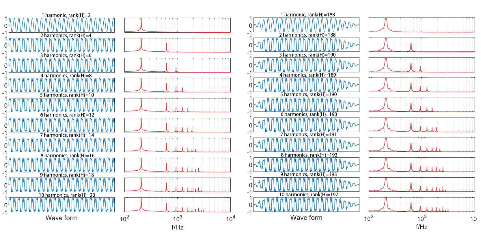
(b) (c) (d)

Figure 4. Low rank properties in audio signals. (a. Wave form of sine wave analogue signals. b. Frequency of sine wave analogue signals. c. Wave form of sine wave analogue signals with envelopes. d. Frequency of sine wave analogue signals with envelopes)

The information perceived by the human ear comes from the frequency domain in which the formants are concentrated, and the formants represent the most direct source of articulatory information, as well as the main feature of speech recognition and the basic information conveyed by speech coding. Accordingly, the low-rank approximation is considered an appropriate methodology for denoising.

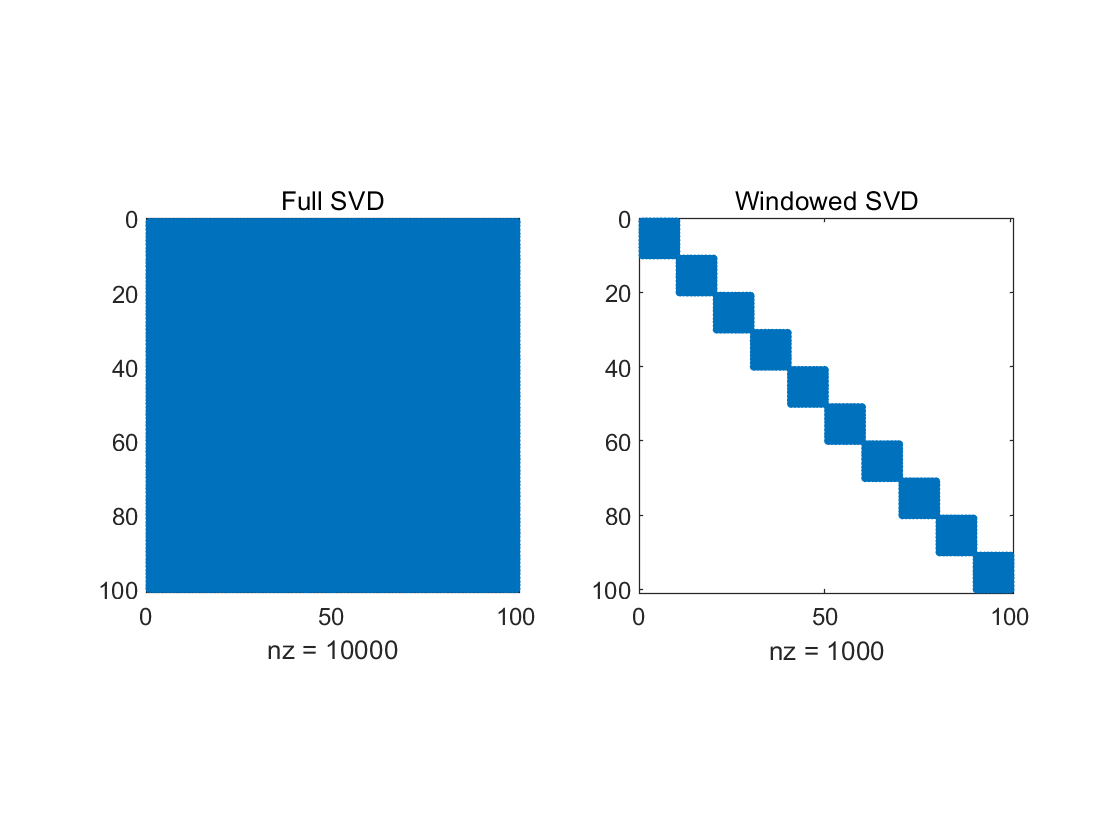
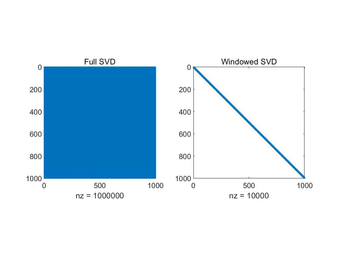
(a) (b)

Figure 5. Memory Space Required for full SVD and WSVD. (a. Data with \( n={10^{4}} \) ; b. Data with \( n={10^{6}} \) )

The main idea of this paper is the frequency partitioning of the signal, coupled with the Lanczos bidiagonalization of the SVD over windows. The former exploits the frequency property of the noise distribution, while the latter exploits the local low-rank nature of the audio signal. Comparing with full SVD, the computational complexity changes from the originally \( O({n^{2}}) \) to \( O(λwn) \) , where \( λ \) , \( w \) are the number of frequency intervals and the window length. Figure 6 represents the actual Hankel matrix sizes that were calculated. Since the denoising process of each window is independent, parallel computations are allowed to further improve the denoising efficiency if the requisite device is available.

5. Conclusion

In this paper, an audio denoising method with WSVD of frequency division is proposed and accelerated by the Lanczos bidiagonalization algorithm for decomposing the first \( k \) large singular values. The algorithm separates noise with audio of different frequency characteristics by splitting the frequency bands, and achieves local low-rank approximation and computational reduction by locally adding windows. Simulation and experimental results show that the frequency-divided WSVD can effectively denoise audio data. Therefore, the algorithm can be applied to many real-life scenarios. Considering that the low-rank approximation of WSVD is a locally linear approximation method, nonlinear approximation of can also be considered in future research.

References

[1]. Florkowski, M. (1999) Wavelet based Partial Discharge Image De-Noising. 1999 Eleventh International Symposium on High Voltage Engineering. London: IEE.
[2]. Zhao, Z.D. (2005) ECG denoising by generalized wavelet shrinkage. ICEMI 2005: Conference Proceedings of the Seventh International Conference on Electronic Measurement & Instruments, 6: 339-342.
[3]. Boyer, R., and Abed-Meraim, K. (2004) Audio Modeling based on Delayed Sinusoids. IEEE Transactions on Speech and Audio Processing. 2(2): 110-120.
[4]. Fevotte, C., and Kowalski, M. (2014) Low-Rank Time-Frequency Synthesis. Advances in Neural Information Processing Systems 27 (NIPS 2014).
[5]. Fevotte, C., and Kowalski, M. (2018) Estimation With Low-Rank Time–Frequency Synthesis Models. IEEE Transactions on Signal Processing, 2018. 66(15):. 4121-4132.
[6]. Yang, Y., and Rao, J. (2019) Robust and Efficient Harmonics Denoising in Large Dataset Based on Random SVD and Soft Thresholding. IEEE ACCESS, 7: 77607-77617.
[7]. Cai, J., Wang, T., and Wei, K. (2019) Fast and Provable Algorithms for Spectrally Sparse Signal Reconstruction via Low-rank Hankel Matrix Completion. Applied and Computational Harmonic Analysis, 46(1): p. 94-121.
[8]. Nguyen, H.M., Peng, X., et al. (2013) Denoising MR Spectroscopic Imaging Data With Low-Rank Approximations.IEEE Transactions on Biomedical Engineering, 60(1): p. 78-89.
[9]. O'Leary, D.P. and Simmons, J.A. (1981) A Bidiagonalization-Regularization Procedure for Large Scale Discretizations of Ill-Posed Problems. SIAM Journal on Scientific and Statistical Computing, 2(4): 474-489.
[10]. Machida, K., Nose, T., and Ito, A. (2014) Speech Recognition in a Home Environment using Parallel Decoding with GMM-based Noise Modeling. 2014: Asia-Pacific Signal and Information Processing Ass.
[11]. Miyake, N., Takiguchi T., and Ariki, Y. (2010) Sudden Noise Reduction Based on GMM with Noise Power Estimation. Journal of Software Engineering and Applications, 2010. 03(04): 341-346.
[12]. Kruczek, P., et al. (2017) The modified Yule-Walker method for α-stable time series models. Physica A: Statistical Mechanics and its Applications, 2017. 469: p. 588-603.
[13]. Middleton, D. (1999) Non-Gaussian noise models in signal processing for telecommunications: new methods an results for class A and class B noise models. IEEE Transactions on Information Theory, 45(4): p. 1129-1149.
[14]. Shibata, R. (1976) Selection of the order of an autoregressive model by Akaike's information criterion. Biometrika, 63(1): p. 117-126.
Cite this article
Li,T. (2024). Fast audio signal denoising with low-rank approximation using windowed singular value decomposition of frequency division. Theoretical and Natural Science,39,268-282.
Data availability
The datasets used and/or analyzed during the current study will be available from the authors upon reasonable request.
Disclaimer/Publisher's Note
The statements, opinions and data contained in all publications are solely those of the individual author(s) and contributor(s) and not of EWA Publishing and/or the editor(s). EWA Publishing and/or the editor(s) disclaim responsibility for any injury to people or property resulting from any ideas, methods, instructions or products referred to in the content.
About volume
Volume title: Proceedings of the 2nd International Conference on Mathematical Physics and Computational Simulation
© 2024 by the author(s). Licensee EWA Publishing, Oxford, UK. This article is an open access article distributed under the terms and
conditions of the Creative Commons Attribution (CC BY) license. Authors who
publish this series agree to the following terms:
1. Authors retain copyright and grant the series right of first publication with the work simultaneously licensed under a Creative Commons
Attribution License that allows others to share the work with an acknowledgment of the work's authorship and initial publication in this
series.
2. Authors are able to enter into separate, additional contractual arrangements for the non-exclusive distribution of the series's published
version of the work (e.g., post it to an institutional repository or publish it in a book), with an acknowledgment of its initial
publication in this series.
3. Authors are permitted and encouraged to post their work online (e.g., in institutional repositories or on their website) prior to and
during the submission process, as it can lead to productive exchanges, as well as earlier and greater citation of published work (See
Open access policy for details).