1. Introduction

In today's globalized economic system, the health and stability of the real estate market is crucial to the development of the social economy. The real estate industry is the foundation and leading industry of a country's national economy, and the housing price has always been one of the issues related to people's livelihood, and the change of housing price is a common phenomenon. The real estate industry directly promotes the development of the economy, and is the main driving force constituting the three growth engines of investment, consumption and import and export [1]. In recent years, governments around the world have introduced relevant policies to regulate and curb the rise of housing prices. As a key indicator to measure market conditions, the fluctuation of housing price not only affects the quality of life of residents, but also an important basis for investors to make decisions [2].

Boston, as a city with a long history and rich educational resources, its real estate market has unique regional characteristics and complex influencing factors. For example, the regional crime rate, the proportion of regional educational resources and other factors have a profound impact on regional housing prices [3]. In addition, this study aims to find the most suitable model for predicting house prices in Boston through advanced data analysis techniques, which not only has important academic value, but also demonstrates the application potential of data science in solving practical problems. Reviewing the valuable research of previous scholars, Zhao used R software to establish a linear regression model for the Boston housing price according to the variables in the Boston housing price data set, and conducted a significance test on the regression equation and regression coefficient. Since the distribution range of the Boston housing price will change with the change of influencing factors, and the median has a certain robustness [4]. Therefore, this paper set up a regression model for the median house price, that is, quantile regression model. The author found that the house price has certain research significance, and there are many models to choose from [5]. As for the selection of the model, Zhang showed in their research on housing prices that through the data analysis and testing, it can be concluded that the multiple linear regression model can effectively predict and analyze housing prices to a certain extent, and the algorithm can still be improved by more advanced machine learning methods [5].

Through the systematic study of the factors affecting the housing price in Boston and the construction of a forecasting model, this study is expected to provide valuable insights and tools for researchers and practitioners in related fields. In recent years, governments around the world have introduced relevant policies to regulate and curb the rise of housing prices [6]. With the acceleration of urbanization and the deepening of regional economic integration, Boston has exhibited unique geographical, economic and social characteristics that have had a profound impact on the real estate market. Based on the conclusion of previous research scholars, the study of housing price fluctuation in the Pearl River Delta one-hour city circle should focus on the economic development situation of the region [7]. The fluctuation of housing prices is influenced to varying degrees by multiple factors, necessitating a comprehensive consideration of these elements in order to effectively regulate housing prices. [8]. It is necessary to study the diversity of factors affecting housing prices. Based on the least square method, this paper establishes and optimizes the multiple linear regression model, conducts real estate price prediction, and finally realizes the functions of housing information retrieval, comparison and data visualization, providing housing price display, analysis and assisted decision-making services for home buyers. Variable selection is always an important research content in statistical analysis and inference [9]. The variables are grouped according to the test results, and the group variables are selected by stepwise regression method. The real variables can be selected from the linear model, the quadratic function model and the complex model, and the validity and feasibility of the new method are verified. The application analysis of the classic Boston house price data shows the practicability of the new method [10].

2. Methodology

2.1. Data source

This part introduces the research object and application method of this paper. All the data used in this paper are from the "Boston House Prices" uploaded by MANIMALA in the Kaggle database, and the data is based on the standard metropolitan area of Boston in 1970.

2.2. Variable description

In the detailed examination of the Boston housing market, the authors adopt a dual-model approach to dissect the complex interplay between diverse socioeconomic factors and the median value of owner-occupied homes (MEDV). Using a multivariate linear regression model, the authors assess the influence of variables such as per capita crime rates (CRIM), residential zoning proportions (ZN), non-retail business acres (INDUS), and various other demographic and geographic characteristics. To capture the intricacies of non-linear relationships and interactions, the authors complement this analysis with a Random Forest model, which leverages the collective wisdom of multiple decision trees to improve predictive accuracy. This combined methodology allows for a more profound examination of the complex effects of factors including the presence of the Charles River (CHAS), nitric oxides concentration (NOX), average room counts (RM), and the socioeconomic status of the population (LSTAT), among others. The study seeks to identify the key drivers of housing prices, providing a refined set of tools for forecasting property market dynamics and guiding strategic choices in the field (Table 1).

Table 1. Explanation of variables.

2.3. Method introduction

Regression analysis is a technique commonly used in statistics that explores potential causal connections between target variables (dependent variables) and explanatory variables (independent variables) by setting these variables. By building a regression model, the writer can use the actual collected data to calculate the individual parameter values in the model. And then evaluate the fit of the model to determine if it accurately reflects the characteristics of the actual data. If the model fits well, then can use the model to combine the values of the independent variables for effective predictive analysis. By reviewing the cases of previous researchers, many methods for housing price prediction have been derived in the field of machine learning. This paper proposes a housing price prediction model based on multivariate regression analysis, adding the current unemployment rate, loan interest rate and national consumption index as variables, which can more effectively fit the data. The experiment selected the housing price of Manhattan from 2010 to 2016 as the data set to predict the local housing price in 2017. The experiment showed that the difference between the predicted price and the real price obtained by the model was about 2%. The model has certain reference value, the experiment is relatively successful, and the model can be used [7].

In this paper, the authors use random forests to rank the importance of eigenvalues to identify the factors that have the most important impact on price. At the same time, a linear regression model and a random forest model were established to predict the housing price, and the coefficient of determination was compared to evaluate the model. By comparing with the absolute percentage error of various types of coal, it can be found that the random forest model generally shows better adaptability and stability [8].

3. Results and discussion

3.1. Descriptive analysis

The table 2 provides a statistical overview of Boston housing market variables, revealing the extremes, averages, and dispersions. For instance, the crime rate ranges widely from 0.00632 to 88.97620, while the average home has about 6.28 rooms. High standard deviations, like 168.537 for property taxes, suggest considerable variation across neighborhoods, essential for gauging market diversity before predictive modeling.

Table 2. Descriptive statistics

3.2. Correlation analysis

By utilizing SPSS, this paper precisely quantified the correlations between variables in the Boston housing dataset, subsequently transforming these numerical insights into a compelling heatmap (Figure 1). In this visual synthesis, the color palette signifies the nature and strength of relationships: deep blues denote strong negative correlations, such as the stark inverse relationship between CRIM and MEDV (-0.385), where higher crime rates correlate with lower housing values. Conversely, intense reds illustrate robust positive correlations, exemplified by the tight association between INDUS and NOX (0.764), indicating that areas with more industrial land also tend to have higher levels of nitrogen oxide. The saturation of hues directly corresponds to the magnitude of correlation coefficients, with darker shades reflecting higher absolute values. This fusion of SPSS analytics with graphical representation not only elucidates the intricate connections within the data but also facilitates a more intuitive grasp of the underlying patterns, critical for refining predictive models and interpreting their outcomes in the context of the housing market.

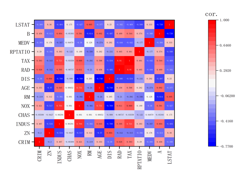
Figure 1. Correlation results.

3.3. Linear model results

Table 3 presents a summary of the multiple linear regression model's performance in predicting Boston housing prices. The R-squared value, standing at 0.525, indicates that the model accounts for approximately 52.5% of the variability in the housing prices, suggesting a moderate level of explanatory power.

Table 3. Linear model results.

The Adjusted R-squared, which is 0.276, adjusts for the number of predictors in the model and suggests that the inclusion of additional variables may not significantly improve the model's fit. The Error value, given as 78.69368, represents the average discrepancy between the predicted and actual housing prices, indicating that there is room for improvement in the model's predictive accuracy. Lastly, the Durbin-Watson statistic, with a value of 0.673, is indicative of potential positive autocorrelation among the residuals, which could imply that the model may not be fully capturing the underlying structure of the data and could benefit from further refinement to enhance its predictive capabilities.

Table 3 provides a statistical breakdown of the coefficients and their significance within the multiple linear regression model used to predict Boston's median housing prices (MEDV). The data reflects several key conclusions about the relationships between the predictors and housing prices.

First, the "Unstandardized Coefficients" (B) reveal the direction and magnitude of each predictor's effect on housing prices. For example, a negative coefficient for CRIM indicates that higher crime rates are associated with lower housing prices, while a positive coefficient for RM suggests that houses with more rooms tend to have higher prices.

Then, the "t" and "Sig." (significance) columns indicate which predictors are statistically significant at the 0.05 level. Predictors with low p-values (e.g., CRIM, RM, TAX, LSTAT) are significantly related to housing prices, suggesting that these variables are important in explaining price variations.

After is the "Tolerance" and Variance Inflation Factor ("VIF") statistics help assess multicollinearity among predictors. High VIF values (e.g., for INDUS, NOX, AGE) suggest that these predictors may be highly correlated with others, which could affect the reliability of their individual coefficients.

Finally, the standardized coefficients (Beta) allow for a comparison of the relative importance of predictors, regardless of their units of measurement. This comparison helps in understanding which variables have a stronger influence on housing prices within the model.

In summary, Table 3 suggests that certain predictors like CRIM, RM, TAX, and LSTAT have a significant impact on Boston's housing prices, while multicollinearity may be an issue with some variables. These insights are valuable for refining the model and for stakeholders to consider when making decisions related to the housing market.

3.4. Random forest results

Table 4 offers a concise ranking of the predictor variables in the Random Forest model, highlighting their relative importance in predicting Boston's median housing prices (MEDV). The "variable" column identifies each predictor, while the "importance" column reflects their contribution to the model's predictive power.

Table 4. Importance rank.

For instance, AGE, with a high importance score, is the top-ranked predictor, indicating that the age of the housing stock significantly influences prices. Conversely, ZN, with a lower or negative importance score, suggests a less significant impact on housing values.

This ranking is crucial for identifying the most influential factors in housing price predictions, aiding stakeholders in making data-driven decisions. It also guides potential refinements to the model, focusing on the most impactful variables.

The graph in figure 2 elegantly illustrates the relationship between the number of prediction samples and a quantitative metric, presumably an indicator of model performance or prediction accuracy. As the sample size increases from 100 to 300 in increments of 100, the corresponding values on the vertical axis range from 50 to 350, suggesting a potential improvement or a different aspect of the model's output that scales with the sample size. This visualization is crucial for understanding how varying the quantity of data affects the predictive capabilities of the model. Figure 6 presents a comparative analysis between different training sets, indicated by the title and the similar scale to figure 2. With the horizontal axis representing the prediction sample size and the vertical axis showing a performance metric, this graph likely aims to reveal any disparities in model training outcomes when different subsets of data are utilized. The consistency in scale with figure 2 allows for a direct comparison, which is essential in evaluating the robustness and generalizability of the model across various data configurations.

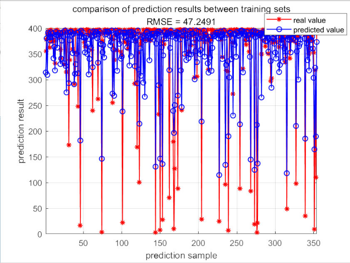
Figure 2. Comparison results of training set.

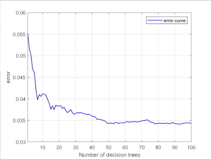
Figure 3. Error curve.

The error curve depicted in figure 3 is a testament to the iterative refinement of a predictive model, possibly a random forest or another ensemble technique. As the number of decision trees increases from 10 to 100, the error rate declines steadily from 0.06 to 0.025, indicating that the model's precision is enhanced with additional trees. This downward-sloping curve is a visual affirmation of the model's learning process, where the complexity of the model is incrementally increased to achieve a lower prediction error. Decision tree model has strong interpretability and is the basis of machine learning methods such as random forest and deep forest [10]. How to select the segmentation attribute and segmentation value of node is the key problem of decision tree algorithm, which affects the generalization ability, depth, balance degree and other important performance of tree.

Figure 4 encapsulates the essence of feature selection in predictive modeling by ranking the importance of various features. The vertical axis, ranging from 0.8 to -0.2, represents the significance of each feature, with higher values indicating a more substantial impact on the model's predictions. This ranking is indispensable for discerning which variables are driving the model's decisions and which may be extraneous or even detrimental to its performance. By identifying the most influential features, this graph guides the model optimization process, ensuring that only the most relevant information is considered in the predictive algorithm.

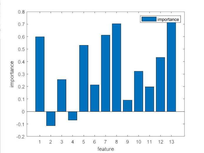
Figure 4. Correlation results.

This paper conducted through the utilization of MATLAB, has yielded a series of metrics that quantify the performance of the predictive model across both training and testing datasets. The Mean Bias Error (MBE) for the training set stands at 0.47844, indicating a relatively small bias in the predictions made during the model's learning phase. Conversely, the MBE for the test set is notably higher at 2.4543, suggesting a greater discrepancy between the predicted and actual values when applied to unseen data, which may indicate overfitting or a lack of generalization.

The coefficient of determination, R², provides insight into the proportion of variance explained by the model. For the training set, R² is 0.73678, signifying that approximately 74% of the variability in the dependent variable is captured by the model. However, the test set's R² of 0.6249 reveals a slight decrease in explanatory power when confronted with new data, a common occurrence as models tend to perform best on the data they were trained on.

Mean Absolute Error (MAE) measures the average absolute difference between predicted and actual values. The training set's MAE, presented in a series of numbers, indicates the average error magnitude for each observation. Similarly, the test set's MAE, also listed numerically, shows the model's accuracy when predicting for fresh instances. Both sets of MAE values offer a granular view of the model's precision across various data points, with higher numbers suggesting larger prediction errors.

Overall, these metrics suggest that while the model performs reasonably well on the training data, there is room for improvement in terms of generalizability and accuracy when applied to new, independent datasets. Further refinement of the model or additional data collection and analysis may help to enhance its predictive capabilities.

4. Conclusion

In the final analysis, the comparative study of the multiple linear regression and Random Forest models for predicting Boston's housing prices has yielded a clear preference for the latter. The Random Forest model, with its ability to capture non-linear relationships and handle high-dimensional data, has consistently outperformed the linear regression model in terms of predictive accuracy, as evidenced by its higher coefficient of determination.

The Random Forest's ensemble approach, which aggregates the predictions of multiple decision trees, has proven adept at discerning the intricate patterns within the Boston housing dataset that are not easily captured by linear models. This superiority is particularly evident in the model's capacity to rank the importance of variables, such as AGE and LSTAT, which emerged as highly influential in predicting housing prices.

While the multiple linear regression model provides valuable insights into linear correlations and is simpler to interpret, its limitations in dealing with complex, non-linear interactions and potential multicollinearity among predictors make it less suitable for this application.

Therefore, based on the empirical evidence and the model's performance metrics, the Random Forest model is the preferred choice for predicting housing prices in Boston. Its robust predictive power and nuanced understanding of the market's complexity make it an invaluable tool for stakeholders seeking to make informed decisions in the dynamic landscape of real estate investment. Future research and applications in this domain should consider the Random Forest model as a powerful and reliable predictive framework.

Authors Contribution

All the authors contributed equally and their names were listed in alphabetical order.

References

[1]. Sheng J and Pan D D 2016 Analysis of influencing factors of housing price based on enhanced regression tree: A case study of Boston area. Statistics and Applications, 5(3), 299-304.
[2]. Li Y Q 2018 Housing price prediction model based on Random forest. Communications World, 306-308.
[3]. Zhao R 2019 Analysis of correlation between house price data in Boston based on regression method. Statistics and Applications, 9(3), 335-344.
[4]. Zhang Q Q 2021 Housing Price Prediction Based on Multiple Linear Regression. SCIENTIFIC PROGRAMMING.
[5]. Yang Y M and Tan S K 2011 Study on the influence of real Estate Price Factors on Housing price and its fluctuation in one hour city circle of the Pearl River Delta. China Land Science, 25(6), 54-59.
[6]. Cao T Y and Chen M Q 2019 Study on random forest variable selection based on studentized range distribution. Statistics and Information Forum, 36(8) 15-22.
[7]. Li S D 2021 Housing price forecasting model based on multivariate linear regression. Science and Technology Innovation, 91-92.
[8]. Guo L, Guo W W 2019 Prediction of thermal coal high calorific value based on SVR and random forest model. Energy Engineering, 44(1), 35-42.
[9]. Wang J T, et al. 2019 Gini Index and decision tree method for mitigating random consistency. Science in China: Information Science, 54(1), 159-190.
[10]. Zheng Y F 2007 Research on the spatial difference of housing prices in different urban areas of Hangzhou. Economic Forum, 32-34.
Cite this article
Jiang,X.;Li,C. (2024). Research on the influencing factors of housing price based on multiple linear regression and random forest. Theoretical and Natural Science,52,49-57.
Data availability
The datasets used and/or analyzed during the current study will be available from the authors upon reasonable request.
Disclaimer/Publisher's Note
The statements, opinions and data contained in all publications are solely those of the individual author(s) and contributor(s) and not of EWA Publishing and/or the editor(s). EWA Publishing and/or the editor(s) disclaim responsibility for any injury to people or property resulting from any ideas, methods, instructions or products referred to in the content.
About volume
Volume title: Proceedings of CONF-MPCS 2024 Workshop: Quantum Machine Learning: Bridging Quantum Physics and Computational Simulations
© 2024 by the author(s). Licensee EWA Publishing, Oxford, UK. This article is an open access article distributed under the terms and
conditions of the Creative Commons Attribution (CC BY) license. Authors who
publish this series agree to the following terms:
1. Authors retain copyright and grant the series right of first publication with the work simultaneously licensed under a Creative Commons
Attribution License that allows others to share the work with an acknowledgment of the work's authorship and initial publication in this
series.
2. Authors are able to enter into separate, additional contractual arrangements for the non-exclusive distribution of the series's published
version of the work (e.g., post it to an institutional repository or publish it in a book), with an acknowledgment of its initial
publication in this series.
3. Authors are permitted and encouraged to post their work online (e.g., in institutional repositories or on their website) prior to and
during the submission process, as it can lead to productive exchanges, as well as earlier and greater citation of published work (See
Open access policy for details).