1. Introduction

For high school students in North America, there are plenty of memorable experiences and memories in the school. Some students make the most significant decisions in high school, such as becoming an occupational basketball player or singer. However, most high school students may choose to continue studying in the universities or colleges they applied to successfully. In this case, academic GPA is significant for high school students in North America because it is an important index for university admissions decisions [1]. GPA in high school can be calculated by all the course scores which are relative to homework and test scores. In this case, most high school students may hope to have a higher GPA to apply to the university. Also, students who have low GPA hope to change their performance to improve their GPA. However, most students with low GPA do not know how to increase their GPA. In this case, most students hope to understand how to get a higher GPA, and which features of students are most important for improving their GPA.

Sawyer found that GPA in high school is useful for universities to predict high school students’ academic success in the future [1]. Kobrin et al. found that the GPA in high school with a correlation of 0.36 is more significant than admission test scores (0.35) in predicting students’ first-year GPA in the university [2]. University of Miami researchers found that a point increase in high school students’ GPA may affect the increasing 12% - 14% of income in the future [3]. In addition, high school GPA is affected by plenty of factors. Philippe et al. proposed that participation in both civic and non-civic organized activities may positively affect students to increase their GPA in high school [4]. Rahafar et al. found that chronotype, gender, conscientiousness, and test may affect high school student GPA, where gender differences had the most impact on students’ GPA by using the structural equation model [5]. Warren showed that students who study in small learning communities could reduce their number of absences and improve their test scores, thereby, increasing their GPA in high school [6]. Therefore, the research plan is to figure out which feature is the most important for affecting high school student’s GPA in North America.

In addition, predicting student’s GPA by their different features without their course scores and homework performance is the main purpose of the research. In this case, the machine learning methods of the research are significant for predicting student’s GPA. Paolo et al. used a logistic multiple regression model to predict the GPA of students and found that cross-validation is important for the generalizability and overall utility of prediction models [7]. Hassan et al. used multiple regression models including linear, ridge, lasso, and LassoCV to predict the GPA of students and found that the LassoCV method is the best model with higher \( {R^{2}} \) and lower RMSE in his dataset selected based on the Community of Inquiry framework [8]. Nasiri et al. utilized regression analysis for predicting GPA and the C5.0 algorithm (a type of decision tree) to predict academic dismissal (Classification Data) [9]. Cai et al. found that gradient boosting regression and random forest models improved by the k-fold cross-validation algorithm are better than other models for predicting net ecosystem carbon exchange (NEE) [10].

Based on their ideas of models for predicting data, the experiment decides to use multiple linear regression, random forest, and boosting models improved by the k-fold cross-validation method to predict high school student’s GPA, thereby, making the comparison between these model methods to choose the best prediction model.

2. Methodology

2.1. Data source

The dataset collection is from Kharoua in Kaggle about features (Student ID, Age, Gender, Ethnicity, Parental Education, Week Study Time, Absences, Tutoring, Parental Support, Extracurricular, Sports, Music, Volunteering, GPA, and Grade Class) of 2392 high school students in North America.

2.2. Dataset preprocessing

For the details of the dataset, data visualization by histograms is necessary for every feature. In this case, a factor (Student ID), which is the ID for all the subjects, having no distribution in the histogram, being not relevant to the value of the GPA of the students (See Figure 1). Therefore, this factor (Student ID) is dropped before predicting the GPA. The other 12 factors' histograms may show that they may affect the GPA (See Figure 2, Figure 3). In addition, Grade Class (Grade Level) is a classification data of GPA, so Grade Level cannot be used to predict GPA. In this case, Grade Level is dropped in the experiment for predicting GPA. Besides, there are data errors and loss that do not exist since the dataset in Kaggle is reprocessed by Kharoua. The only problem with the dataset is that students’ GPA in this dataset are relatively low since Kharoua might collect the data from most students with bad academic performance. The boxplot is necessary for finding outliers for numeric factors but all numeric data in this dataset do not have outliers through the boxplot (See Figure 4). Also, the experiment normalizes 12 factors’ data (except Student ID, GPA, and Grade Class) in the dataset to eliminate data differences between factors.

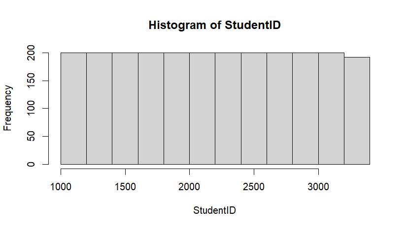
Figure 1. Histogram of Student ID.

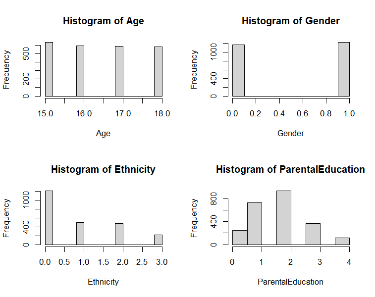
Figure 2. Histogram of age, gender, ethnicity, and parental education.

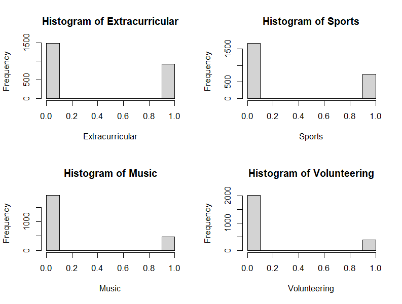
Figure 3. Histogram of extracurricular, sports, music, and volunteering.

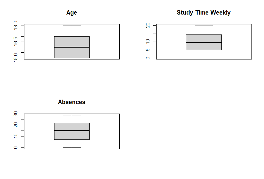
Figure 4. Box plot of age, study time weekly, absences.

2.3. Variable selection

The experiment has already dropped 3 factors to have the 12 dataset factors as the variables including Age, Gender, Ethnicity, Parental Education, Week Study Time, Absences, Tutoring, Parental Support, Extracurricular, Sports, Music, and Volunteering. In this case, the experiments make variables have their logograms (See Table 1).

Table 1. Logogram of the 12 factors and target factor.

2.4. Method introduction

The experiment utilizes a correlation matrix to determine the feature importance in the dataset. Before creating models to predict GPA, the dataset is divided into two datasets which are the model train dataset (80%) and the test dataset (20%). The experiment trains multiple linear regression models as the base model for predicting the GPA and uses the cross-validation and stepwise regression methods to improve the regression model. For the 12 factors in the model, the multilinearity check is necessary for having a good regression model. In addition, the experiment may use random forest and boosting to create models to compare with the multiple linear regression models to determine the best model for predicting students’ GPA. Finally, the experiment calculates the value of mean squared error (MSE) and \( {R^{2}} \) from every model for comparison between models. In addition, using the confusion matrix by predicting model data checks every model's accuracy.

3. Results and discussion

3.1. Descriptive analysis

The experiment describes the information of 12 factors and target variable from the original dataset, which includes name, mean, standard deviation (SD), median, trimmed mean (Trimmed), median absolute deviation (Mad), minimum (Min), maximum (Max), range, and standard error (SE) (See Table 2). In addition, the experiment uses the 12 factors' histograms to analyze their distribution.

Table 2. Factor information.

3.2. Correlation analysis

For correlation between the factors and GPA, the correlation matrix is a good method to check which factor is the most important for predicting GPA. In this dataset, the figure shows that absences with a correlation (- 0.92) have the most impact on GPA, which is negatively correlated with students’ GPA (See Figure 5).

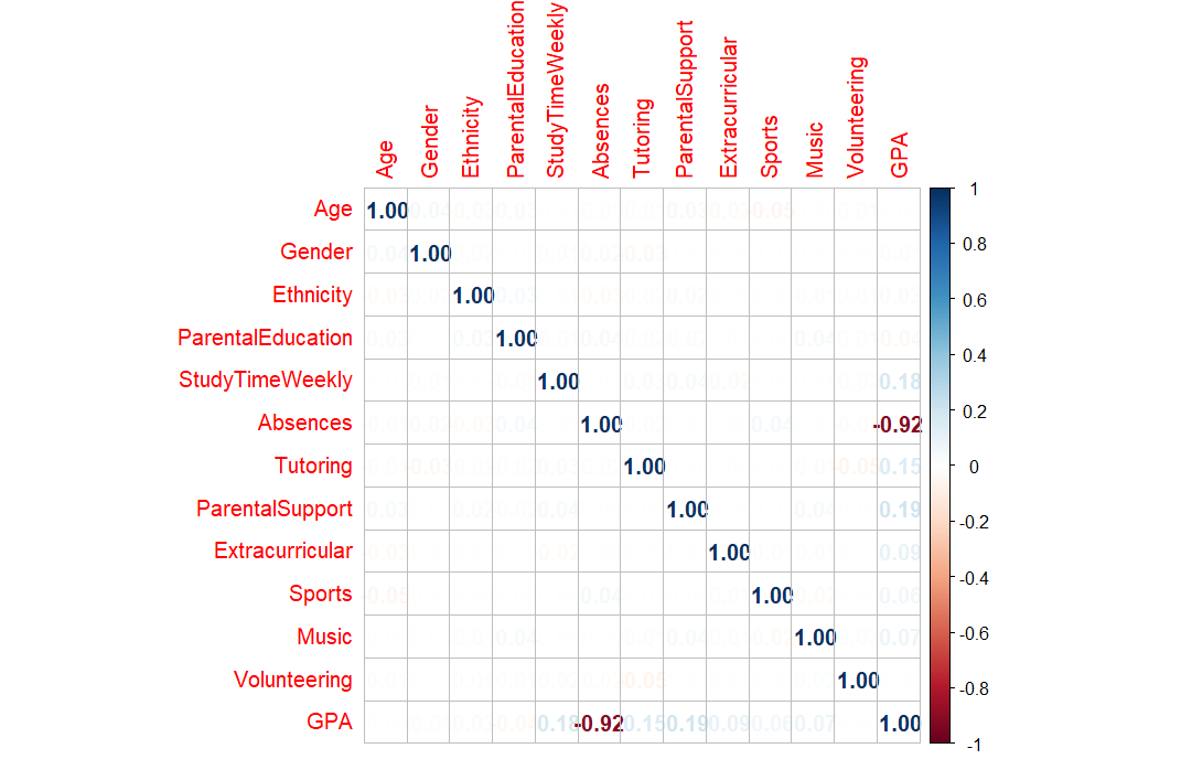
Figure 5. Correlation plot.

3.3. Model analysis

3.3.1. Multiple linear regression model 1. The experiment uses the training dataset to create a multiple linear regression model (Model 1) between 12 factors and GPA first (See Table 3).

Table 3. Summary of Model 1

3.3.2. Global validation linear model assumption. In this case, the experiment uses the global validation of the linear model assumption function to check whether the experiment needs to improve the linear regression model (See Table 4). In Table 4, the assumption of global stat and skewness is not satisfied, then it shows that some factors do not have a linear relationship with students’ GPA.

Table 4. GVLMA of Model 1

3.3.3. Multicollinearity check of Model 1. Checking multicollinearity by using the Durbin-Watson Test (DW test), variance inflation factor (VIF), and kappa coefficient is necessary for finding some factors with autocorrelation. Therefore, there is no multicollinearity in this model because DW test value =1.9664, VIF < 2, and value of kappa < 5 (See Table 5).

Table 5. Value of VIF

3.3.4. Stepwise regression of model 2. The stepwise regression method is a good idea to reduce several useless factors to create a new linear regression model (Model 2) (See Table 6). In Table 6, the stepwise regression model reduces four factors (Parental Education, Ethnicity, Volunteering, and Gender) to have a new linear regression model.

Table 6. Summary of Model 2

3.3.5. Simple linear regression model 3. Figure 2 and Figure 3 show that Absences are the most impact factor for GPA, so it is meaningful for the experiment to create a simple linear regression model (Model 3) between Absences and GPA (See Table 7).

Table 7. Summary of Model 3

3.3.6. Stepwise linear regression model 4 by 10-fold cross-validation. Table 3 shows that the p-value of five factors (Age, Gender, Ethnicity, Parental Education, and Volunteering) is larger than 0.05, which means that they are not significant for the model. In this case, the experiment utilizes the stepwise regression method by the 10-fold cross-validation to train a new multiple linear regression model (Model 4) (See Table 8).

Table 8. Summary of Model 4

3.3.7. Random forest model 5 and 6. Except for the multiple linear regression model, the experiment chooses to use the random forest method to train a new model (Model 5) with all 12 factors for predicting GPA. In addition, Model 4 shows that there are several factors (Age, Gender, Ethnicity, Parental Education, and Volunteering) are dropped, so the experiment trains a relative model (Model 6) with 7 factors left by using the random forest.

3.3.8. Boosting model 7 and 8. Boosting is a good regression method for predicting GPA in this dataset, so a new boosting model (Model 7) is trained with 12 factors. In addition, the experiment trains a relative boosting model (Model 8) with 7 factors left, since the experiment dropped 5 factors in Model 4.

3.4. Comparison analysis

The experiment predicts the value of GPA by different models, thereby, calculating MSE and \( {R^{2}} \) by using the prediction data and the test dataset (See Table 9). The experiment uses the prediction of GPA value and test dataset round to the nearest single digit to calculate the accuracy of every model through the confusion matrix (See Table 9).

Table 9. Comparison of Models

Compared with other models, Model 4 with only 7 factors has 84.03% accuracy which is the most accurate for predicting Grade Level (See Table 9). Also, Model 1 has the lowest MSE (0.0386) and highest \( {R^{2}} \) (95.6%), slightly better than Model 4 in predicting GPA. However, Model 1 is trained by using all 12 factors, which is more complex than Model 4. In this case, the experiment chooses to use Model 4 as the best model in the research (See Function of Model 4 below). Function of Model 4 (See Table 8) (Round to three decimal places):

\( y=0.585{x_{5}}-2.891{x_{6}}+0.247{x_{7}}+0.599{x_{8}}+0.196{x_{9}}+0.195{x_{10}}+0.143{x_{11}}+2.519\ \ \ (1) \)

By using the same dataset in Kaggle, Knapp showed that the support vector machine (SVM) is the best model to predict the Grade Level (classification data of GPA), which has 74.5% accuracy. Compared with his experiment results, Model 4 with 84.03% accuracy in the experiment has increased almost 10% accuracy for predicting Grade Level.

3.5. Resident test of model 4

The experiment chooses Model 4 to be the best model in this research, so the experiment needs to use the test plot to check the model assumptions including normal independent identically distribution errors, constant error variance, absence of influential cases, linear relationship between predictors and the outcome variable, and collinearity (See Figure 6). Figure 6 shows that Model 4 successfully passes these five tests. Therefore, Model 4 is a good model that does not need to be optimized deeply.

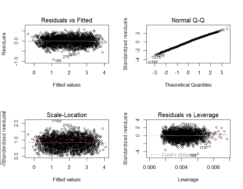
Figure 6. Residual test of Model 4

4. Conclusion

The research works on predicting high school students’ GPA by the experiment above. The experiment uses three machine learning methods to train 8 regression models to find the best model for predicting GPA and Grade Level. In this case, Model 4 with 7 factors is the most simple and accurate regression model in the experiment (See the function of Model 4 in the Result). Therefore, Model 4 is useful and important for school administrators to estimate the GPA of students. Also, the experiment can let students know which should be improved to increase their GPA.

For the experiment, several places can be improved in the future. Firstly, subjects in the dataset are not large enough (only 2000+), which may decrease the accuracy of models for predicting data. In addition, plenty of features from students, which is not in this dataset, may significantly affect the GPA in high school, such as subject learning abilities, mental health, and social support. For the machine learning methods, the experiment only uses three different methods, especially for using only one method from the random forest or boosting method. In this case, the research can use more regression methods to train more models to have the best model for predicting the GPA in the future.

References

[1]. Sawyer R 2013 Beyond Correlations: Usefulness of High School GPA and Test Scores in Making College Admissions Decisions. Applied Measurement in Education, 26(2), 89-112.
[2]. Kobrin J L, et al. 2008 Validity of the SAT® for Predicting First-Year College Grade Point Average. Research Report, College Board.
[3]. Miami U O 2014 New Research Shows How Students' High School GPA Could Affect Their Income. Lab Manager.
[4]. Philippe F L, et al. 2023 Organized civic and non-civic activities as predictors of academic GPA in high school students. Applied Developmental Science, 27(2), 189-204.
[5]. Rahafar A, Maghsudloo M, Farhangnia S, Vollmer C and Randler C 2015 The role of chronotype, gender, test anxiety, and conscientiousness in academic achievement of high school students. Chronobiology International, 33(1), 1-9.
[6]. Warren J E 2016 Small Learning Communities and High School Academic Success. ProQuest Dissertations & Theses.
[7]. Paolo A M, Bonaminio G A, Durham D and Stites S W 2004 Comparison and Cross-validation of Simple and Multiple Logistic Regression Models to Predict USMLE Step 1 Performance. Teaching and Learning in Medicine, 16(1), 69-73.
[8]. Hassan Y M I, Elkorany A and Wassif K 202. Utilizing Social Clustering-Based Regression Model for Predicting Student’s GPA. IEEE Access, 10, 48948-48963.
[9]. Nasiri M, Minaei B and Vafaei F 2012 Predicting GPA and academic dismissal in LMS using educational data mining: A case mining. 6th National and 3rd International Conference of E-Learning and E-Teaching, 53-58.
[10]. Cai J, Xu K, Zhu Y, Hu F and Li L 2020 Prediction and analysis of net ecosystem carbon exchange based on gradient boosting regression and random forest. Applied Energy, 262, 114566.
Cite this article
Zhu,W. (2024). High school student GPA prediction by various linear regression models. Theoretical and Natural Science,52,153-162.
Data availability
The datasets used and/or analyzed during the current study will be available from the authors upon reasonable request.
Disclaimer/Publisher's Note
The statements, opinions and data contained in all publications are solely those of the individual author(s) and contributor(s) and not of EWA Publishing and/or the editor(s). EWA Publishing and/or the editor(s) disclaim responsibility for any injury to people or property resulting from any ideas, methods, instructions or products referred to in the content.
About volume
Volume title: Proceedings of CONF-MPCS 2024 Workshop: Quantum Machine Learning: Bridging Quantum Physics and Computational Simulations
© 2024 by the author(s). Licensee EWA Publishing, Oxford, UK. This article is an open access article distributed under the terms and
conditions of the Creative Commons Attribution (CC BY) license. Authors who
publish this series agree to the following terms:
1. Authors retain copyright and grant the series right of first publication with the work simultaneously licensed under a Creative Commons
Attribution License that allows others to share the work with an acknowledgment of the work's authorship and initial publication in this
series.
2. Authors are able to enter into separate, additional contractual arrangements for the non-exclusive distribution of the series's published
version of the work (e.g., post it to an institutional repository or publish it in a book), with an acknowledgment of its initial
publication in this series.
3. Authors are permitted and encouraged to post their work online (e.g., in institutional repositories or on their website) prior to and
during the submission process, as it can lead to productive exchanges, as well as earlier and greater citation of published work (See
Open access policy for details).