1. Introduction

From the aspect of the global situation, the COVID-19 pandemic since 2019 precipitated an unprecedented global economic downturn, with far-reaching impacts on various sectors, including the energy market. The initial outbreak led to widespread lockdowns, factory shutdowns, and reduced transportation activities, culminating in a dramatic drop in industrial and commercial energy demand. As a result, the consumption of natural gas would experience frequent changes. Therefore, in such an environment, it is essential to capture the major trend of consumption of natural gas for several purposes such as energy market stability, supply chain management, governmental policy about energy, etc.

Natural gas, as a widely used fossil fuel, many scholars have researched the topic of the market of natural gas. Botão believed that, although the liquefied natural gas (LNG) market will face challenges such as supply-demand imbalances and competition from renewable energy sources, the market will continue to grow and evolve in the future [1]. Further, Qian stated that the transition to clean and low-carbon energy is an unstoppable global trend, and LNG will play an increasingly important role in the international energy mix, while several of the world's major natural gas suppliers have successfully seized the industry opportunity to compete for the dominant position in global LNG supply [2]. In addition, Anam suggested that climate change and global warming have been at the top of the list of issues facing several countries over the past few years, and as a result, many countries have begun to look for alternative sources of energy that can meet their cumulative energy needs, and natural gas is one of those choices [3]. Consequently, the author considers natural gas as an important role in the energy market and the demand for such clean energy continues to grow, which emphasizes the essence of a precise and reliable forecast of natural gas consumption whether in the long-term or the short-term.

In the study of forecasting natural gas consumption, several distinct methods and models were used in scholars' research. Wang et al. established a novel grey model with seasonal dummy variables to predict the seasonal fluctuations of U.S. natural gas consumption [4]. In addition, the particle swarm optimization algorithm was used to attain the optimal approximate time response formula in the forecasting [4]. Liang et al. used the product partition model (PPM) to eliminate the change points in the consumption series and established the Markov switching (MS) model to capture the phase trials of the adjusted series [5]. Lu et al. improved and used a kernel-based nonlinear extension of the Arps decline model for the forecasting [6]. Galadima and Aminu used a structural vector autoregression (SVAR) model with sign restriction to identify the effects of macroeconomic variables on natural gas consumption [7]. Besides, some scholars attempted to apply machine learning techniques in the prediction. Singh et al. applied a machine learning model of artificial neuron network (ANN) and support vector machine (SVM) to forecast annual natural gas consumption in U.S [8]. Wei et al. established an artificial intelligence white-box forecasters model which is a hybrid model consisting of the following methods: principal component analysis (PCA), weighted parallel model architecture (WPMA) and multiple linear regression (MLR), to provide interpretable forecasts for daily natural gas consumption [9]. Qiao et al. predicted natural gas consumption in the short-term based on the Volterra adaptive filter and improved whale optimization algorithm [10]. In addition, the autoregressive integrated moving average (ARIMA), which is a widely used model in time series forecasts, was also considered to apply. Akpinar and Yumusak trained ARIMA model on monthly household natural gas consumption series with training set from 2009 to 2012, and the optimal ARIMA parameters for minimum mean absolute percentage error (MAPE) were found [11]. Pradhan et al. applied ARIMA model in the prediction of Indian natural gas consumption, with goodness of fit statistics checked [12].

In summary, the consumption of natural gas is an important data related to the global energy market while scholars have developed statistical models and artificial intelligence methods for forecasting. This article will treat the natural gas consumption data as a time series such that the time series analysis technique can be applied. Further, the article will use ARIMA model to capture the short-term characterizations of the consumption time series.

2. Methodology

2.1. Data source

The data is collected from Federal Reserve Economic Data (FRED), including a time series of monthly consumption of natural gas in billion cubic feet. Further, the dataset was recorded on the first day of each month from 2000.1.1 to 2024.5.1, and it consists of 297 observations.

2.2. Variable selection

In the article, monthly natural gas consumption in billion cubic feet is considered as variable. As figure 1 shown, the time series plot provided depicts monthly natural gas consumption in billion cubic feet from 2000.1.1 through 2024.5.1. The vertical axis represents the time-axis and the horizontal axis represents consumption in billion cubic feet.

In the early 2000s, when the series began, natural gas consumption fluctuated above and below around 1500 billion cubic feet, with significant seasonal variations and occasional peaks. Over the years, a general upward trend can be observed, indicating a steady increase in consumption.

Between 2000 and 2005, natural gas consumption remained relatively stable with periodic peaks and troughs reflecting seasonal demand patterns. From 2005 onwards, baseline consumption gradually increased, interspersed with seasonal fluctuations.

A more pronounced upward trend began around 2010, with consumption levels reaching higher peaks and no longer declining during the off-peak seasons. This trend continues until it becomes more pronounced after 2015, when consumption continues to rise and reach new highs.

By 2020, natural gas consumption peaks near 300 Bcf and seasonal variations, while still present, are less pronounced relative to overall growth. This trend continues through 2024, when consumption reaches its highest level, suggesting that natural gas use has continued to rise over a 24 year (Figure 1).

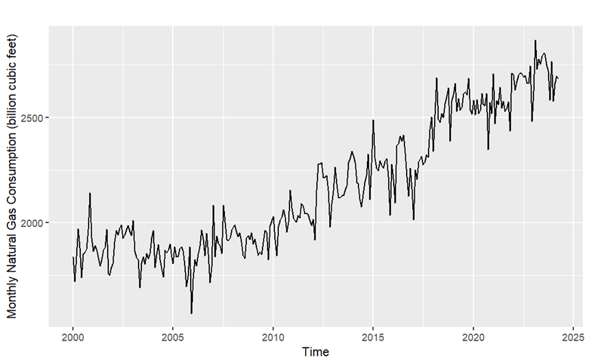
Figure 1. Monthly Natural gas Consumption (billion cubic feet).

2.3. Model selection

Based on the research of Akpinar et al., ARIMA model was shown to be feasible in the prediction of consumption of natural gas [11]. Therefore, the article considers ARIMA model to forecast on the consumption time series.

ARIMA model is a widely used model in time series analysis and forecasts. It is a composition of following models and methods: autoregression (AR) model, integral (I) method and moving average (I) model. Mathematically, the ARIMA model is given by:

\( y_{t}^{ \prime }=c+\sum _{i=1}^{p}{ϕ_{i}}y_{t-i}^{ \prime }+\sum _{j=1}^{q}{θ_{j}}{ϵ_{t-j}}+{ϵ_{t}} \) (1)

where \( y_{t}^{ \prime } \) is the differenced series and the degree of difference is denoted as \( d \) . Further, \( {ϵ_{t}} \) denotes the error. \( {ϕ_{i}} \) and \( {θ_{j}} \) are autoregressive parameters and moving average parameters respectively. \( c \) is a constant. The ARIMA model given by the equation above, with \( p \) autoregressive parameters, \( d \) -th order differencing and \( q \) moving average parameters is called ARIMA(p,d,q) model.

3. Results and discussions

3.1. Data preprocess

Stability is one of the most important characteristics to verify whether a model is appropriate or not for a time series. As the figure 2 illustrated, the dataset shows a significant positive autocorrelation for all considered \( k \) -values, i.e. \( k = 1,2,…,24 \) . Obviously, the consumption series is non-stationary. Taking differenced series is suggested to obtain stationary data.

Figure 3 shows the ACF of the differenced series. By taking differenced, most of the autocorrelation values lie within the critical value (blue-dashed lines) as figure 3 shown. To further examine the stationary of the differenced series, unit root test was used. In the report, the Kwiatkowski-Phillips-Schmidt-Shin (KPSS) test was considered, which is a type of unit root test with null hypothesis to be trend stationarity [13]. The corresponding test-statistic is 0.0316, which is small enough to imply the stationary of the differenced series.

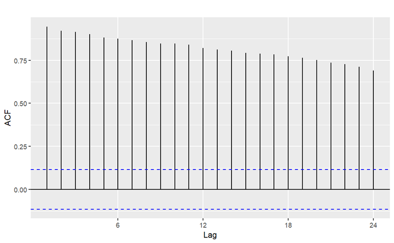
Figure 2. Autocorrelation function (ACF) plot of the consumption series.

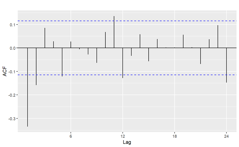
Figure 3. Partial autocorrelation function (PACF) plot of the consumption series.

3.2. Model parameters determination

The ARIMA model is consisting of three crucial parameters, i.e. \( (p,d,q) \) as section 2.3 discussed (Table 1). In this section, the parameters \( p \) and \( q \) were obtained by minimizing two statistic metrics among, Akaike information criterion (AIC), while parameter \( d \) was determined in the previous subsection, with \( d=1 \) .

Figure 4 shows the PACF of the differenced series and it is used in approximate the parameter of the ARIMA model based on time series analysis. The PACF shown in figure 4 suggests an ARIMA(2,1,0) model since there are the autocorrelation values for lag 1 and 2 are significant, which implies a strong correlation of the time series with the second-order lag series. Therefore, ARIMA(2,1,0) and its closed variations (ARIMA models with similar \( (p,q) \) -parameters) were considered. Further, their AIC values are computed to compare their performance on the series (as table 2 shown). According to the results in table 2, ARIMA(1,1,1) attains the minimized AIC among the candidate models. Therefore, it is sufficient to believe that the ARIMA(1,1,1) is most appropriate ARIMA model based on the statistical properties of the consumption data. In addition, the fitting coefficients of ARIMA(1,1,1) are shown in table 3.

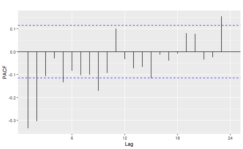
Figure 4. Partial autocorrelation function (PACF) plot of the differenced consumption series.

Table 1. AIC comparation of distinct ARIMA models

Table 2. Fitting coefficients of ARIMA(1,1,1) models.

3.3. Model evaluation

To verify whether the selected model is reliable, the residual of the model would be examined to check if its residual is white noise. The results of the above test are shown in figure 5. As the ACF plot in the figure shown, majority of the autocorrelation lies in the critical region with a few spikes nearly reaches the critical bound. In addition, the histogram of the residual illustrated that the residual distribution is closed to normal distribution. Therefore, the article can consider the residual of the model cannot be distinguishable from the white noise. As a result, ARIMA (1,1,1) is reliable enough to make a further forecast for the consumption series.

ARIMA (1,1,1) model is considered to predict 12 numerical values (one year) for natural gas consumption data. The numerical result is shown in table 3 and forecast plot is shown in figure 5 and 6. The blue line indicates the forecast values from the model and the black line indicates the recorded consumption data. Based on the model prediction, for the next year, the consumption of natural gas stays constant level with a slight fluctuation.

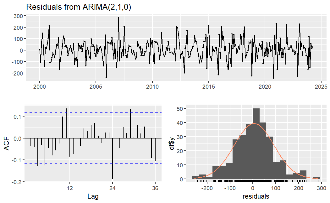
Figure 5. Residual plot of the model (top), ACF plot of the model (bottom left) and distribution of the residual (bottom right).

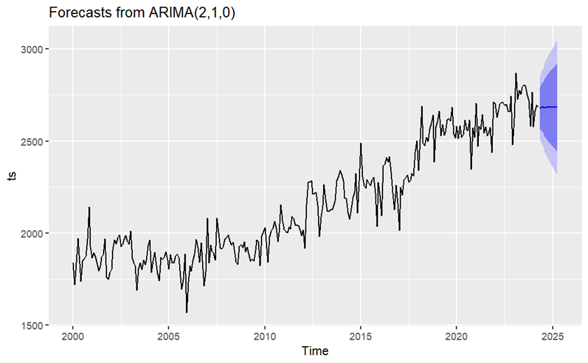
Figure 6. Forecast plot of ARIMA (1,1,1)

3.4. Further discussion

Through the conclusion in precious part, the natural gas consumption reaches a stable level in the short-term, implying that there would not be any significant changes or influence on the natural gas market.

Although the considered model has a certain degree of reliability due to the verified statistical metrics and tests as previous subsection shown, some problems are above the context of the article. First of all, the consumption of natural gas should follow some cyclic properties with annual periods because of factors such as heating demand at winter and seasonal industrial demand fluctuations. However, the ARIMA model fails to capture such trial. Secondly, despite that the prediction capture the short-term trend as figure 7 illustrated, it seems fail to demonstrate the long-term uplifting trend as figure 6 shown (Table 3). Therefore, certain limitations of the model and predictions are occurred in this article.

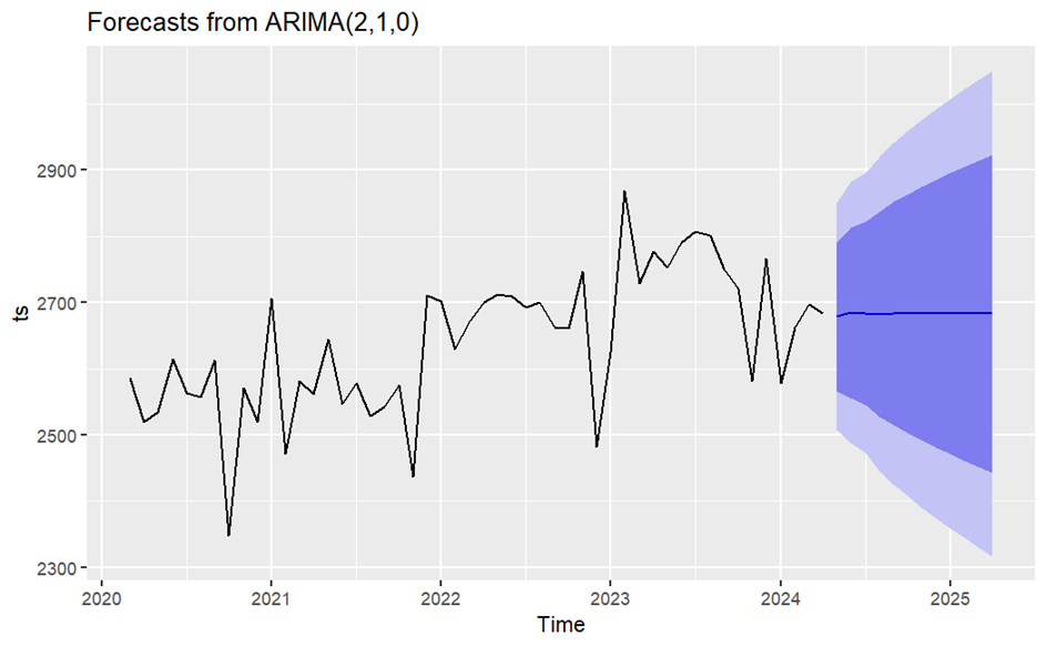
Figure 7. Forecast plot (zoomed) of ARIMA (1,1,1)

Table 3. Numerical forecast result from ARIMA (1,1,1)

4. Conclusion

Through the research in this article, it can be concluded that natural gas consumption in U.S. would stay still for future one year, while the overall trend of consumption is increasing. However, the prediction would be inaccurate to some degree since various factors, such as natural gas situation, weather variation and global economics etc. have not been considered in constructing the model.

Based on the prediction and long-term trend, the article suggests that long-term investment in natural gas-related industrial is recommended. Besides, short-term investment that is shorter than a year can also be considered although the benefit is not considerable compared to long-term due to the invariant consumption as the prediction demonstrated.

Finally, the ARIMA model cannot capture the annual cycle characteristics of the series. For further research, the improvement of ARIMA model such as seasonal ARIMA (SARIMA) model, ARIMA with external data (ARIMAX) is suggested. Furthermore, alternative models such as error, trend, seasonal state space (ETS) model can be also considered. The above-stated models are able to capture seasonality of cycle characteristics and the long-term trend of the series.

References

[1]. [1] Botão R P, De Medeiros Costa H K and Dos Santos E M 2023 Global gas and LNG markets: demand, supply dynamics, and implications for the future. Working paper.
[2]. [2] Zou Q, Yi C, Wang K, Yin X and Zhang Y 2022 Global LNG market: supply-demand and economic analysis. IOP Conf. Series: Earth and Environmental Science, 983(1), 12051.
[3]. [3] Azam A, Rafiq M, Shafique M, Zhang H and Yuan J 2021 Analyzing the effect of natural gas, nuclear energy and renewable energy on GDP and carbon emissions: A multi-variate panel data analysis. Energy, 219, 119592.
[4]. [4] Wang Z, He L and Zhao Y 2021 Forecasting the seasonal natural gas consumption in the US using a gray model with dummy variables. Applied Soft Computing, 113, 108002.
[5]. [5] Liang T, Chai J, Zhang Y and Zhang Z 2019 Refined analysis and prediction of natural gas consumption in China. Journal of Management Sci. and Engr, 4(2), 91-104.
[6]. [6] Lu H, Ma X and Azimi M 2020 US natural gas consumption prediction using an improved kernel-based nonlinear extension of the Arps decline model. Energy, 194, 116905.
[7]. [7] Galadima M D and Aminu A W 2019 Shocks effects of macroeconomic variables on natural gas consumption in Nigeria: Structural VAR with sign restrictions. Energy Policy, 125, 135-144.
[8]. [8] Singh S, Bansal P, Hosen M and Bansal S K 2023 Forecasting annual natural gas consumption in USA: Application of machine learning techniques- ANN and SVM. Resources Policy, 80, 103159.
[9]. [9] Wei N, Yin L, Li C, Li C, Chan C and Zeng F 2021 Forecasting the daily natural gas consumption with an accurate white-box model. Energy, 232, 121036.
[10]. [10] Qiao W, Yang Z, Kang Z and Pan Z 2020 Short-term natural gas consumption prediction based on Volterra adaptive filter and improved whale optimization algorithm. Engr. Apl. of Artificial Intelligence, 87, 103323.
[11]. [11] Akpinar M and Yumusak N 2013 Forecasting household natural gas consumption with ARIMA model: A case study of removing cycle. 2013 7th Int. Conf. on Apl. of Information and Communication Technologies, 1-6.
[12]. [12] Kumar P, Dhal S and Kumar N 2017 Neural network based forecasting model for natural gas consumption. Communications on Applied Electronics, 7(11), 1-8.
[13]. [13] Xiao Z 2001 Testing the null hypothesis of stationarity against an autoregressive unit root alternative. Journal of Time Series Analysis, 22(1), 87-105.
Cite this article
Huang,W. (2024). Forecast of consumption of natural gas in U.S. based on time series analysis and ARIMA model. Theoretical and Natural Science,51,157-164.
Data availability
The datasets used and/or analyzed during the current study will be available from the authors upon reasonable request.
Disclaimer/Publisher's Note
The statements, opinions and data contained in all publications are solely those of the individual author(s) and contributor(s) and not of EWA Publishing and/or the editor(s). EWA Publishing and/or the editor(s) disclaim responsibility for any injury to people or property resulting from any ideas, methods, instructions or products referred to in the content.
About volume
Volume title: Proceedings of CONF-MPCS 2024 Workshop: Quantum Machine Learning: Bridging Quantum Physics and Computational Simulations
© 2024 by the author(s). Licensee EWA Publishing, Oxford, UK. This article is an open access article distributed under the terms and
conditions of the Creative Commons Attribution (CC BY) license. Authors who
publish this series agree to the following terms:
1. Authors retain copyright and grant the series right of first publication with the work simultaneously licensed under a Creative Commons
Attribution License that allows others to share the work with an acknowledgment of the work's authorship and initial publication in this
series.
2. Authors are able to enter into separate, additional contractual arrangements for the non-exclusive distribution of the series's published
version of the work (e.g., post it to an institutional repository or publish it in a book), with an acknowledgment of its initial
publication in this series.
3. Authors are permitted and encouraged to post their work online (e.g., in institutional repositories or on their website) prior to and
during the submission process, as it can lead to productive exchanges, as well as earlier and greater citation of published work (See
Open access policy for details).