1. Introduction

The Maxwell’s equations are a set of partial differential equations that describe the interrelationship between electric and magnetic fields. Discretization methods for solving Maxwell’s equations include finite difference methods , finite volume methods [1-3], spectral methods [4], and finite element methods [5-13]. In 2014, Brenner, Gedicke, and Sung extended the Hodge decomposition method to two-dimensional time-harmonic Maxwell’s equations with anisotropic permittivity and impedance boundary conditions [14]. They derived error estimates for the P1 finite element method based on Hodge decomposition and presented numerical experimental results for metamaterials and electromagnetic cloaking. The main idea of this thesis originates from Brenner, Gedicke, and Sung’s proposal to convert Maxwell’s equations into standard second-order elliptic boundary value problems based on Hodge decomposition, and then to solve them using standard nodal finite element discretization methods. Therefore, after obtaining the numerical solution in this paper, it is post-processed using conventional techniques, specifically the Superconvergent Patch Recovery (SPR) and Polynomial Preserving Recovery (PPR) methods, to improve the approximation accuracy of the curl and bcurl of the numerical solution.

2. Statement of the result

This paper employs a node adaptive finite element method based on Hodge decomposition to solve the two-dimensional Maxwell’s equations. The advantages of using this approach are: 1. It transforms the solution of Maxwell’s equations into the solution of standard elliptic boundary value problems, for which there are very mature algorithms. 2. Compared to edge element basis functions, the computation involving node basis functions is more cumbersome and computationally intensive; hence, this method simplifies the computation.

The essence of solving the two-dimensional Maxwell’s equations in this paper is to address a standard second-order scalar elliptic boundary value problem. Therefore, after converting Maxwell’s equations into a standard second-order scalar elliptic boundary value problem using the Hodge decomposition method, a nodal finite element method is applied to find the solution. The numerical solution obtained for the elliptic boundary value problem, \( {ϕ_{h}},{φ_{j,h}},{c_{j,h}}, \) is then used to derive the numerical solution for Maxwell’s equations \( {u_{h}}=∇×{ϕ_{h}}+\sum _{i=1}^{m}{c_{i,h}}{φ_{i,h}}. \) The numerical solution \( {u_{h}} \) is piecewise constant, thus finite element gradient reconstruction techniques such as SCR (Superconvergent Patch Recovery) and PPR (Polynomial Preserving Recovery) are utilized to effectively enhance the precision of the numerical solution. Based on the research presented, this paper establishes a reliable a posteriori error indicator and an adaptive finite element method. For simplicity, the dielectric constant and permeability in the numerical experiments are set to 1, and the boundary conditions are assumed to be perfectly conducting, which, as demonstrated by the results of the examples, improves the rate of convergence.

In this paper, the dielectric constant and permeability are taken as 1, and Maxwell’s’s equations are considered with perfectly conducting boundaries. Future research can continue to explore the node adaptive finite element analysis based on Hodge decomposition for Maxwell’s’s equations with general dielectric and magnetic properties. Moreover, since this paper addresses the two-dimensional Maxwell’s equations, it is also feasible to consider applying the node adaptive finite element method based on Hodge decomposition to investigate the three-dimensional Maxwell’s equations in the future.

3. Preliminaries

3.1. Maxwell’s equations

\( ∇×E=-\frac{∂B}{∂t}, \) (2.1)

\( ∇×H=J+\frac{∂D}{∂t}, \) (2.2)

\( ∇\cdot D=q, \) (2.3)

\( ∇\cdot B=0, \) (2.4)

The Maxwell’s equations comprehensively and specifically describe the three fundamental laws of electromagnetism: Gauss’s law, Ampère’s law, and Faraday’s law. Here, \( E \) represents the electric field, \( H \) the magnetic field, \( D \) the electric flux density, \( B \) the magnetic flux density, and \( J \) the current density; all are functions of time \( t \) and space \( x \) . \( q \) is the charge density, a scalar quantity. By definition, moving charges generate currents, and the continuity equation can explain the relationship between \( J \) and \( q \) .

\( ∇\cdot J=-\frac{∂q}{∂t}. \) (2.5)

The solution of Maxwell’s equations also requires the following interface conditions:

\( n×E=0, \) (2.6)

\( n×H={J_{s}}, \) (2.7)

\( n\cdot D={q_{s}}, \) (2.8)

\( n\cdot B=0, \) (2.9)

Here, \( {q_{s}} \) is the external surface charge density on the boundary surface, and \( {J_{s}} \) is the external surface current density on the boundary surface. When it is an insulating medium, \( {q_{s}}=0 \) and \( {J_{s}}=0 \) .

To avoid using two unknowns, one can eliminate \( E(orD) \) or \( H(orB) \) from Maxwell’s equations to obtain the main research model of this paper. The derivation process of this model is referenced in [15]. The model studied in this paper has only one unknown \( E \) and the model is given below:

\( ∇×{μ^{-1}}∇×E-{κ^{2}}(ϵE)=f, in Ω, \) (2.10)

\( n×E=0, on ∂Ω, \) (2.11)

where \( E∈{H_{0}}(curl;Ω)∩H(di{v^{0}};Ω;ϵ), \) and \( f \) is the current density.

3.2. Two-dimensional hodge decomposition

3.2.1. Properties of two-dimensional divergence-free and curl-free vector fields

A vector field \( v∈{[{L^{2}}(Ω)]^{2}} \) satisfies \( ∇\cdot v=0, ⟨v\cdot n,1{⟩_{{Γ_{j}}}}=0,0≤j≤n, \) if and only if there exists a function \( ϕ∈{H^{1}}(Ω) \) such that \( v=∇×ϕ, \) where \( ∇×ϕ=(\frac{∂ϕ}{∂{x_{2}}},-\frac{∂ϕ}{∂{x_{1}}}) \) [16]. Moreover, the uniqueness of \( ϕ \) is determined by a constant.

Note 1 If the region \( Ω \) is simply connected then \( v=∇×ϕ \) if and only if \( ∇\cdot v=0. \)

A vector field \( v∈{[{L^{2}}(Ω)]^{2}} \) satisfies \( ∇×v=0,⟨v\cdot t,1{⟩_{{Γ_{j}}}}=0,0≤j≤n, \) if and only if there exists a function \( ϕ∈{H^{1}}(Ω) \) such that \( v=∇ϕ, \) where \( t \) is a unit tangent vector [16]. In addition, the uniqueness of \( ϕ \) is determined by a constant.

3.2.2. Hodge decomposition

The following introduces the Hodge decomposition. The decomposition of \( H(di{v^{0}};Ω;ϵ) \) is as follows:

\( H(di{v^{0}};Ω;ϵ)=K+H, \) (2.12)

Where

\( K={ϵ^{-1}}∇×{H^{1}}(Ω)=\lbrace {ϵ^{-1}}∇×ϕ:ϕ∈{H^{1}}(Ω)\rbrace , \)

\( H=∇×H(Ω;ϵ)=\lbrace ∇×ϕ:ϕ∈H(Ω;ϵ)\rbrace . \)

3.3. Finite element gradient recovery

Finite element recovery technology is a post-processing method, mainly to obtain an improved solution, which is obtained by reconstructing the finite element solution. Finite element recovery can not only obtain better gradient approximation but also perform error estimation. SCR Recovery and PPR Recovery are Gradient Recovery which employ post-processing methods based on the least squares approach.

SCR Recovery The SCR method involves reconstructing the gradient of the finite element solution by fitting a linear polynomial to the solution values at nodes surrounding a particular node of interest, using the least squares technique. This method is advantageous because it provides a Superconvergent gradient approximation, which can be used for error estimation and mesh refinement in adaptive finite element methods.

PPR Recovery The PPR method, on the other hand, fits a quadratic polynomial to the solution values at nodes in the vicinity of a node of interest. This process requires at least six nodes to perform the fitting. The PPR method is known for preserving the polynomial nature of the solution, which means that if the true solution is a polynomial of a certain degree, the PPR method will exactly reproduce this polynomial within the patch. This property makes PPR particularly useful for maintaining the accuracy of the solution in regions where the solution behaves polynomially.

Comparing the definitions of SCR and PPR reveals their main differences.

SCR selects sample points that are symmetrically distributed around the point of reconstruction, with at least four points required. It fits a linear polynomial to the function values at these nodes using the least squares method and then uses the derivatives of this polynomial to obtain the recovered gradient. This method is relatively simple in terms of computation and implementation.

PPR, in contrast, requires the selection of no fewer than six nodes that do not lie on a single quadratic curve. It involves fitting a quadratic polynomial \( {p_{2}} \) to the nodes and their function values through a local least squares approach. The gradient of this polynomial is then used to recover the numerical solution’s gradient at the point of interest, \( ({G_{h}}{u_{h}})(z)=∇{p_{2}}(z), \) and it maintains the polynomial nature of the solution [17]. Due to the higher degree of the polynomial and the larger number of nodes involved, PPR involves more computational work and has a more complex procedure compared to SCR.

4. Numerical Examples

This chapter presents various analytical solutions for different domains. Error figures are provided to assess the accuracy of the method. The parameters are set as \( μ,κ,ϵ=1 \) for simplicity and to facilitate the comparison of results.

The computational domain is taken as \( Ω={(0,4)^{2}}\{[1,3]^{2}}, \) The right-hand side term is a discontinuous function:

\( f(x)=\begin{cases}\begin{matrix}[1+x,0], & x \lt y,3 \lt x \lt 4, \\ [0,1+y], & else. \\ \end{matrix}\end{cases} \)

Utilizing Hodge decomposition for the discrete solution of the equation yields graphical results.

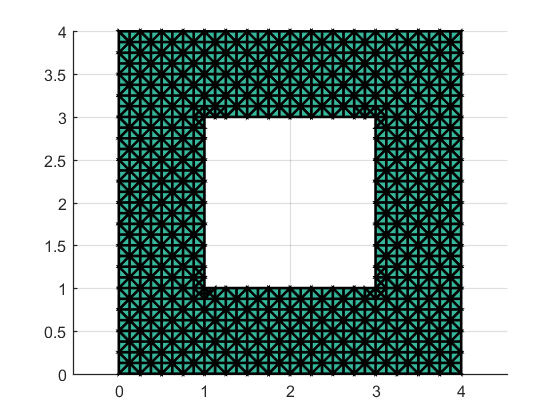
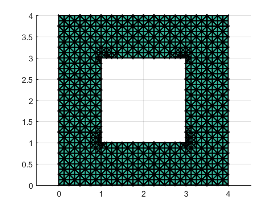
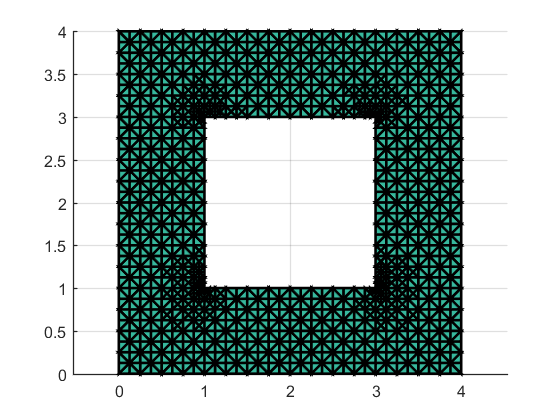
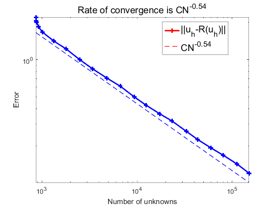
Figures 1 to 3 are the diagrams obtained from the adaptive mesh refinement performed 2, 3, and 4 times, respectively. Figure 4 is the error convergence order of the recovery indicator. Since the right-hand side term \( f \) is known in this example, but the true solution is unknown, the error convergence order between the true solution and the numerical solution cannot be determined. The region is a non-simply connected domain, and during adaptive refinement, it is evident that the mesh is refined at the four inner corners, with an error convergence order of \( O(h). \)

5. Conclusion

This paper presents a novel approach to solving two-dimensional Maxwell's equations by transforming them into standard elliptic boundary value problems using the Hodge decomposition method. By employing a node finite element method, the proposed approach circumvents the typical issues associated with edge elements, such as a high number of degrees of freedom and poor condition numbers in the resulting linear systems. The incorporation of Superconvergent Patch Recovery (SCR) and Polynomial Preserving Recovery (PPR) post-processing techniques further enhances the accuracy of the numerical solutions, yielding reliable results that are validated by four representative examples. The significance of this study lies in its potential to streamline and improve numerical solutions to Maxwell's equations, especially in cases with perfectly conducting boundaries. By relying on well-established methods for elliptic boundary value problems, this approach contributes a computationally viable alternative to traditional edge finite elements, broadening the scope for numerical applications in electromagnetic field modeling. However, this work also has certain limitations. The analysis is confined to two-dimensional Maxwell's equations and assumes a dielectric constant and permeability of one, with perfectly conducting boundaries. Future research could extend this approach to three-dimensional problems and explore scenarios with variable dielectric and magnetic properties. Additionally, further refinement of the adaptive strategy could be pursued to optimize computational efficiency, particularly in more complex boundary conditions and material configurations.

References

[1]. V. Shankar, H. Mohammadian, F. Hall. A time-domain finite-volume treatment for the Maxwell’s equations[J]. Electromagnetics, 1990, 10:127-145.
[2]. Y. Q. Huang, J. C. Li. Time-domain finite element methods for Maxwell’s equations in meta-materials[M]. Berlin:Springer, 2013.
[3]. F. Hermeline. A finite volume method for solving Maxwell’s equations in inhomogeneous media on arbitrary meshes[J]. Comptes Rendus Mathematique, 2004, 339(12): 893-898.
[4]. Y. X. Liu, J. Lee, T. Xiao. A spectral-element time-domain solution of Maxwell’s equation[J]. Microwave and Optical Technology Letters, 2006, 48(4): 673-681.
[5]. S. Durand, M. Slodicka. Fully discrete finite element method for Maxwell’s equations with nonlinear conductivity[J]. IMA Journal of Numerical Analysis, 2011, 31(4): 1713-1733.
[6]. S. Durand, M. Slodic˘ka. Convergence of the mixed finite element method for Maxwell’s equations with nonlinear conductivity[J]. Mathematical Methods in the Applied Sciences, 2012, 35(13): 1489-1504.
[7]. H. Y. Duan, F. Jia, P. Lin. The local L2 projected C0 finite element method for Maxwell problem[J]. SIAM Journal on Numerical Analysis, 2009, 47(2): 1274-1303.
[8]. P. Ciarlet, J. Zou. Fully discrete finite element approaches for time-dependent Maxwell’s equations[J]. Numerische Mathematik, 1999, 82(2): 193-219.
[9]. L. Wang, Q. Zhang, Z. Zhang. Superconvergence analysis and PPR recovery of arbitrary order edge elements for Maxwell’s equations[J]. Journal of Scientific Computing, 2019, 78(2): 1207-1230.
[10]. C. Yao, S. Jia. Asymptotic expansion analysis of nonconforming mixed finiteelement methods for time-dependent Maxwell’s equations in debye medium[J]. Applied Mathematics and Computation, 2014, 229: 34-40.
[11]. A. Hazra, P. Chandrashekar, D. S. Balsara. Globally constraint-preserving FR/DG scheme for Maxwell’s equations at all orders[J]. Journal of Computational Physics, 2019, 394: 298-328.
[12]. V. A. Rukavishnikov, A. O. Mosolapov. Weighted edge finite element method for Maxwell’s equations with strong singularity[J]. Doklady Mathematics, 2013, 87(2): 156-159.
[13]. P. Hansbo, T. Rylander. A linear nonconforming finite element method for Maxwell’s equations in two dimensions Part I:frequency domain[J]. Journal of Computational Physics, 2010, 229(18): 6534-6547.
[14]. S. C. Brenner, J. Gedicke, L. Y. Sung. Hodge decomposition for two-dimensional time-harmonic Maxwell’s equations:impedance boundary condition[J]. Mathe-matical Methods in the Applied Sciences, 2017, 40(2): 370-390.
[15]. M. G. Larson, F. Bengzon. The finite element method:theory, implementation, and applications[M]. Berlin:Springer, 2013.
[16]. Z. Nan. Application of Helmholtz/Hodge decomposition to finite element methods for two-dimensional Maxwell’s equations[D]. Louisiana State University and Agricultural and Mechanical College, 2013.
[17]. C. Carstensen, S. Bartels. Each averaging technique yields reliable a posteriorierror control in FEM on unstructured grids Part I:low order conforming, nonconforming, and mixed FEM [J]. Mathematics of Computation, 2000, 71(20): 945-970.
Cite this article
Wang,Y. (2025). Node Adaptive Finite Element Method Based on Hodge Decomposition for 2D Maxwell’s Equation. Theoretical and Natural Science,86,139-144.
Data availability
The datasets used and/or analyzed during the current study will be available from the authors upon reasonable request.
Disclaimer/Publisher's Note
The statements, opinions and data contained in all publications are solely those of the individual author(s) and contributor(s) and not of EWA Publishing and/or the editor(s). EWA Publishing and/or the editor(s) disclaim responsibility for any injury to people or property resulting from any ideas, methods, instructions or products referred to in the content.
About volume
Volume title: Proceedings of the 4th International Conference on Computing Innovation and Applied Physics
© 2024 by the author(s). Licensee EWA Publishing, Oxford, UK. This article is an open access article distributed under the terms and
conditions of the Creative Commons Attribution (CC BY) license. Authors who
publish this series agree to the following terms:
1. Authors retain copyright and grant the series right of first publication with the work simultaneously licensed under a Creative Commons
Attribution License that allows others to share the work with an acknowledgment of the work's authorship and initial publication in this
series.
2. Authors are able to enter into separate, additional contractual arrangements for the non-exclusive distribution of the series's published
version of the work (e.g., post it to an institutional repository or publish it in a book), with an acknowledgment of its initial
publication in this series.
3. Authors are permitted and encouraged to post their work online (e.g., in institutional repositories or on their website) prior to and
during the submission process, as it can lead to productive exchanges, as well as earlier and greater citation of published work (See
Open access policy for details).