


1. Introduction
In today’s financial environment, accurately predicting stock market prices presents a significant economic challenge. The volatility and complexity of financial markets require advanced analytical methods for effectively forecasting future price movements. While traditional statistical methods have been effective, they often struggle to capture the inherent nonlinear patterns and long-term dependencies in financial time-series data. To address these complex issues, machine learning techniques, particularly Recurrent Neural Networks (RNNs) and their variants, have gained increasing importance.
Recurrent Neural Networks (RNNs) are a class of neural networks designed to recognize patterns in data sequences, such as time series. Among the various types of RNNs, Long Short-Term Memory (LSTM) networks have received significant attention for their ability to retain information over extended periods. This capability is particularly valuable in financial time-series forecasting, where past events can significantly influence future trends.
The primary objective of this study is to accurately predict stock market prices using LSTM networks. The significance of addressing this issue lies in its potential impact on investment strategies, risk management, and economic stability. LSTM networks are more effective at modeling the complex temporal dependencies present in financial data than traditional methods. Therefore, addressing this problem offers multiple benefits, providing substantial advantages for individual investors, financial institutions, and the broader economy. Accurate predictions can lead to more informed investment decisions, optimizing returns and minimizing investor risk. Additionally, it enhances the ability of financial institutions to develop robust trading algorithms and strategies, ultimately contributing to the efficiency and stability of financial markets.
2. Literature Review
In recent years, with the rapid development of deep learning technology, many scholars have explored its application in financial time-series forecasting, particularly through the use of RNN and LSTM models for stock price prediction. Selvin et al. [1] proposed a sliding window model based on LSTM, RNN, and CNN for stock price prediction. Using minute-level stock data from the National Stock Exchange (NSE) of India, they compared the performance of the three deep learning models and found that the CNN performed best at capturing market dynamics. Sunny, Maswood, and Alharbi [2] developed a stock price prediction framework using LSTM and Bidirectional LSTM (BI-LSTM) models. Their research showed that BI-LSTM outperformed traditional LSTM models in prediction accuracy. Jeenanunta, Chaysiri, and Thong [3] studied the use of LSTM and Deep Belief Network (DBN) models to predict the daily stock prices of the top five companies listed on Thailand’s SET50 index. The results indicated that the LSTM model performed better at predicting low-volatility stocks, while DBN excelled at predicting high-volatility stocks. Srivastava and Mishra [4] proposed an improved LSTM model for predicting the stock prices of Tesla Inc., demonstrating that the LSTM model had superior accuracy compared to traditional methods such as simple averaging, linear regression, and ARIMA. Wang, Liu, Wang, and Liu [5] explored the application of the LSTM algorithm in stock market prediction and significantly improved prediction accuracy by optimizing the gradient descent algorithm and using dropout techniques. Patel, Patel, and Darji [6] compared the performance of RNN and LSTM models in stock price prediction, finding that RNN outperformed LSTM in terms of accuracy. Zhang, Gu, Chang, and Ye [7] proposed a model combining Deep Belief Networks (DBN) and LSTM to predict stock price fluctuations, demonstrating that this combined model significantly outperformed traditional methods in prediction performance through experiments involving 36 Chinese A-share companies. Finally, Zhao, Zeng, Liang, Kang, and Liu [8] proposed a stock price trend prediction model based on RNN, LSTM, and GRU, incorporating an attention mechanism to improve model performance. Their research showed that the GRU and LSTM models significantly outperformed RNN in prediction accuracy, with the inclusion of the attention mechanism further improving prediction precision.
3. Methodology
3.1. Model Overview
In this study, we employed a deep learning model based on Long Short-Term Memory (LSTM) neural networks to predict stock prices. LSTM networks are widely recognized for their ability to effectively capture both long-term dependencies and short-term fluctuations in time series data, making them particularly suitable for sequence prediction tasks. We implemented the LSTM model using the PyTorch framework, leveraging its robust computational capabilities and flexible model definition features to ensure optimal performance and scalability.
3.2. Data Preprocessing
Data preprocessing is a critical step in ensuring the success of the model. First, we selected a set of feature columns from the raw dataset that were deemed valuable for prediction. These columns reflect the main trends and fluctuations in the historical price data. Subsequently, we split the dataset into training and test sets using the train_test_split function from the sklearn library. This division is crucial for validating the model on different data, thereby avoiding overfitting.
Before feeding the data into the model, it is typically normalized to scale the features to a standard range (e.g., 0 to 1), which enhances the stability and convergence speed of model training. Additionally, we employed a sliding window method to generate time series inputs. This method involves creating input sequences, each containing a continuous segment of time data mapped to the corresponding target price.
3.3. Model Architecture
The LSTM model is composed of the following key components:
3.3.1. LSTM Layer
The LSTM layer is the core component of the model, responsible for processing the input time series data and capturing temporal dependencies. The LSTM layer uses a gating mechanism that controls the flow of information, such as the Input Gate, Forget Gate, and Output Gate. These gates collectively determine how information is updated at each time step.
The mathematical formulas for an LSTM unit are as follows:
\( {i_{t}}=σ({W_{i}}\cdot [{h_{t-1}},{x_{t}}]+{b_{i}}) \)
\( {f_{t}}=σ({W_{f}}\cdot [{h_{t-1}},{x_{t}}]+{b_{f}}) \)
\( {o_{t}}=σ({W_{o}}\cdot [{h_{t-1}},{x_{t}}]+{b_{o}}) \)
\( {\widetilde{C}_{t}}=tanh({W_{C}}\cdot [{h_{t-1}},{x_{t}}]+{b_{C}}) \)
\( {C_{t}}={f_{t}}*{C_{t-1}}+{i_{t}}*{\widetilde{C}_{t}} \)
\( {h_{t}}={o_{t}}*tanh({C_{t}}) \)
Where:
\( {i_{t}} \) is the Input Gate, controlling the extent to which new information enters the cell state.
\( {f_{t}} \) is the Forget Gate, determining which information in the current cell state needs to be discarded.
\( {o_{t}} \) is the Output Gate, controlling the influence of the cell state on the hidden state output.
\( {C_{t}} \) is the cell state, storing the long-term dependencies of the time series.
\( {h_{t}} \) is the hidden state, containing the output information passed from the previous time step to the next.
3.3.2. Linear Layer
After the LSTM layer processes the data, the output is passed through a linear layer. The linear layer maps the LSTM output to predict the stock price. This layer typically performs a linear regression operation, represented by the formula:
\( {y_{t}}=W\cdot {h_{t}}+b \)
Where \( {y_{t}} \) is the predicted stock price, \( W \) is the weight matrix, \( {h_{t}} \) is the hidden state output from the LSTM layer, and \( b \) is the bias term.
3.4. Training Process
The model’s training process involves the following key steps:
3.4.1. Loss Function
Mean Squared Error (MSE) was used as the loss function to measure the difference between predicted and actual stock prices. The formula for MSE is:
MSE= \( \frac{1}{n}\sum _{i=1}^{n}({y_{i}}{-{\hat{y}_{i}})^{2}} \)
Where \( {y_{i}} \) is the actual stock price, \( {\hat{y}_{i}} \) is the predicted price, and \( n \) is the number of samples.
3.4.2. Optimizer
To optimize the model parameters, we used the Adam optimizer, which is known for its efficiency and adaptive learning rate properties. Adam combines the advantages of the momentum method and RMSProp, allowing it to adjust the learning rate dynamically for each parameter based on the first and second moments of the gradients. This ensures faster convergence and better stability during training.
The Adam optimizer updates the model’s weights using the following formulas:
\( {m_{t}}={β_{1}}{m_{t-1}}+(1-{β_{1}}){g_{t}} \)
\( {v_{t}}={β_{2}}{v_{t-1}}+(1-{β_{2}}){g_{t}} \)
\( {\hat{m}_{t}}=\frac{{m_{t}}}{1-β_{1}^{t}}, {\hat{v}_{t}}=\frac{{v_{t}}}{1-β_{2}^{t}} \)
\( {θ_{t}}={θ_{t-1}}-α\frac{{\hat{m}_{t}}}{\sqrt[]{{\hat{v}_{t}}}+ϵ} \)
Where:
\( {g_{t}} \) is the gradient at time step t;
\( {m_{t}} \) is the exponentially decaying average of past gradients (momentum);
\( {v_{t}} \) is the exponentially decaying average of past squared gradients;
\( {\hat{m}_{t}} \) and \( {\hat{v}_{t}} \) are bias-corrected estimates;
\( α \) is the learning rate;
\( {θ_{t}} \) represents the model parameters being updated;
3.4.3. Training and Validation
The model was trained on the training set, and its performance was validated using the test set. The training process involved multiple iterations (epochs) until the loss function converged to an acceptable level. After each epoch, the model’s performance was evaluated on the validation set to ensure it did not overfit and could generalize well to unseen data.
In summary, this methodology provides a detailed explanation of the technical implementation of the LSTM-based stock price prediction model, including data preprocessing, model architecture, mathematical principles, and key steps in the training process. Using these methods, we developed a deep learning model that effectively predicts stock prices.
4. Results
In this experiment, we used the historical stock prices of Tesla Inc. (TSLA) over a 10-year period. The dataset was sourced from Yahoo Finance, a trusted source of financial data. The dataset includes daily records of Tesla’s stock prices, covering the opening price, highest price, lowest price, closing price, adjusted closing price, and trading volume.
This dataset provides a comprehensive view of Tesla’s stock performance over a significant period, making it well-suited for long-term trend analysis and predictive modeling.
4.1. Identifying Feature and Label Columns
In this step, we defined the combinations of feature columns (factors) and label columns (target variables) for our predictive modeling experiment. The objective was to explore how different feature combinations influence the accuracy of predicting Tesla’s stock price.
• Feature Columns (F): These are the inputs to our model used to learn and make predictions.
• Label Columns (L): These are the outputs or target variables that the model aims to predict.
The columns are labeled as follows(example):
Table 1: Example labeled columns
Date | Open(1) | High(2) | Low(3) | Close(4) | Adj Close(5) | Volume(6) |
2010-06-29 | 19 | 25 | 17.54 | 23.89 | 23.89 | 18766300 |
• F1: Open Price - The price at which the stock opened on a given day.
• F2: High Price - The highest price reached during the day.
• F3: Low Price - The lowest price reached during the day.
• F4: Close Price - The price at which the stock closed on a given day.
• F5: Adjusted Close Price - The closing price adjusted for splits and dividends.
• L1: Close Price - Used as a label in one of the setups.
• L4: Close Price - Used as a label in another setup.
We tested two different setups:
4.1.1. Setup A
• Feature Columns: F1, F2, F3, F4 (Open, High, Low, Close)
• Label Column: L1 (Close Price)
• Representation: (F1, F2, F3, F4) → L1
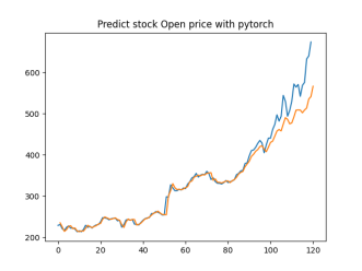
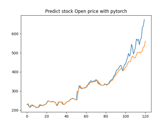
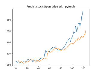
In this setup, we used the stock’s opening, highest, lowest, and closing prices as features to predict the next day’s closing price. This setup examines how these primary trading metrics can predict the closing price.
4.1.2. Setup B
• Feature Columns: F1, F2, F3, F4, F5 (Open, High, Low, Close, Adjusted Close)
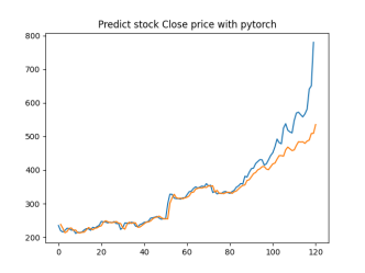
• Label Columns: L1 (Close Price), L4 (Close Price)
• Representation: (F1, F2, F3, F4, F5) → (L1, L4)
These setups allowed us to compare the effectiveness of different feature combinations in predicting the stock’s closing price. We assessed the performance of each setup using the Mean Squared Error (MSE), training loss, and validation loss.
4.2. Determine the Suitable “Time Step”
In this step, we experimented with different time steps to determine the most effective window of historical data for predicting Tesla’s stock price. The time steps tested were 20, 30, 40, 50, and 60 days. The goal was to identify the time step that minimized the Mean Squared Error (MSE), training loss, and validation loss.
Table 2: Performance Metrics Across Time Steps
Time Step | A: (F1 - F4) - L1 | B: (F1 - F5) - L1&L4 | ||||
| MSE | Train loss | Valid loss | MSE | Train loss | Valid loss |
20 | 0.06561169 | 0.002442 | 0.001591 | [0.05275779 0.12036391] | 0.0032 | 0.002221 |
30 | 0.04700987 | 0.002275 | 0.001337 | [0.05503776 0.10871002] | 0.002957 | 0.002055 |
40 | 0.05845572 | 0.002408 | 0.001552 | [0.05964431 0.1225173] | 0.002875 | 0.002235 |
50 | 0.06196832 | 0.002181 | 0.001286 | [0.0594098 0.13030252] | 0.00289 | 0.002057 |
60 | 0.05386019 | 0.002406 | 0.001352 | [0.04302618 0.10403401] | 0.002895 | 0.001946 |
Results
• Setup A (F1, F2, F3, F4) → L1:
• Time Step 30:
• MSE: 0.04701
• Train Loss: 0.002275
• Valid Loss: 0.001337
• Setup B (F1, F2, F3, F4, F5) → (L1, L4):
• Time Step 30:
• MSE: [0.05503776, 0.10871002]
• Train Loss: 0.002957
• Valid Loss: 0.002055
A time step of 30 days emerged as optimal for both setups, showing the lowest MSE, training loss, and validation loss. This suggests that 30 days of historical data offers a balanced and efficient window for predicting Tesla’s stock price.
4.3. Select the Time Period for Stock Prices
We evaluated the model’s performance across different time periods to determine the most suitable range of historical data for predicting Tesla’s stock price. The time periods tested were:
• Half-year (0.5 year): August 2019 - January 2020
• 1 year: February 2019 - January 2020
• 2 years: February 2018 - January 2021
• 5 years: February 2015 - January 2020
• 10 years: January 2010 - December 2019
Table 3: Performance Metrics Across Different Historical Time Periods
Years | A: (F1 - F4) - L1 | B: (F1 - F5) - L1&L4 | ||||
| MSE | Train loss | Valid loss | MSE | Train loss | Valid loss |
0.5 | 1.83508375 | 0.02465 | 0.025958 | [2.15312831 2.58944325] | 0.031666 | 0.031304 |
1 | 1.70008188 | 0.020882 | 0.021573 | [2.05613878 2.46843996] | 0.022363 | 0.023355 |
2 | 1.62572682 | 0.01991 | 0.016375 | [1.56691839 2.54057025] | 0.022356 | 0.019774 |
5 | 0.33621527 | 0.008519 | 0.006221 | [0.50689581 0.98420885] | 0.01201 | 0.009851 |
10 | 0.04700987 | 0.002275 | 0.001337 | [0.05503776 0.10871002] | 0.002957 | 0.002055 |
Results
• Setup A (F1, F2, F3, F4) → L1:
• 10 Years:
• MSE: 1.514898
• Train Loss: 0.016772
• Valid Loss: 0.014656
• Setup B (F1, F2, F3, F4, F5) → (L1, L4):
• 10 Years:
• MSE: [1.331109, 2.001251]
• Train Loss: 0.020389
• Valid Loss: 0.016543
The 10-year period emerged as the optimal choice for both setups, demonstrating the lowest MSE, train loss, and validation loss. This result indicates that the longest available historical data provides sufficient context for accurate predictions, capturing both short-term fluctuations and long-term trends.
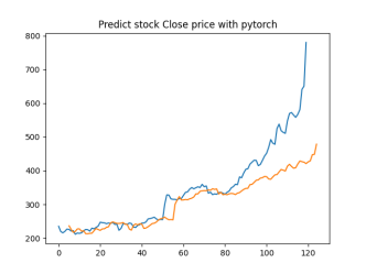
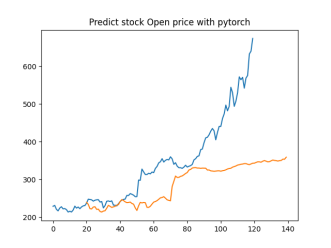
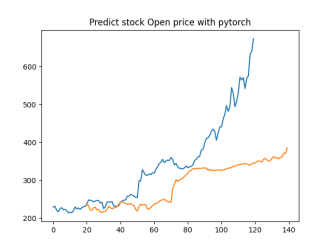
4.4. Varying Prediction Days
In this step, we analyzed how the model’s predictions for Tesla’s stock price varied with different prediction horizons. The prediction days tested were 1, 5, 10, 15, 20, 25, and 30 days.
Table 4: Performance Metrics Across Different Prediction Days
Prediction days | (F1 - F4)L1 - A | (F1 - F5)L1&L4 - B | |
| Open | Open | Close |
1 | MSE: 0.04401224
| MSE: 0.05880658
| MSE: 0.12691709
|
5 | MSE: 0.22312771
| MSE: 0.27531077
| MSE: 0.35481763
|
10 | MSE: 0.53628417
| MSE: 0.53810132
| MSE: 0.60469295
|
15 | MSE: 0.66894851
| MSE: 0.69096178
| MSE: 0.78858355
|
20 | MSE: 0.84486569
| MSE: 0.8356581
| MSE: 0.94040684
|
25 | MSE: 0.92773771
| MSE: 0.96346316
| MSE: 1.04912824
|
30 | MSE: 1.0968706
| MSE: 1.11719375
| MSE: 1.22853315
|

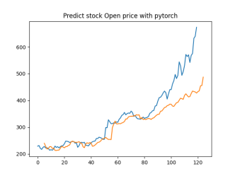
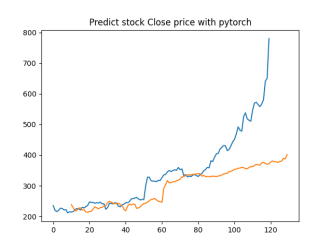

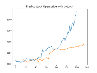


Analysis
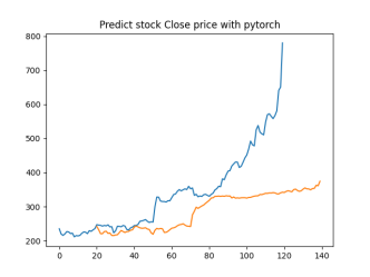
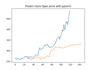
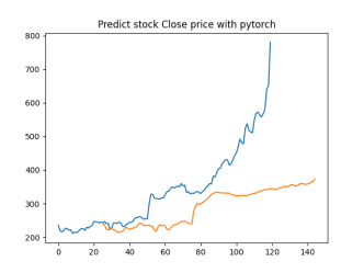
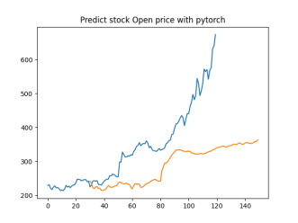
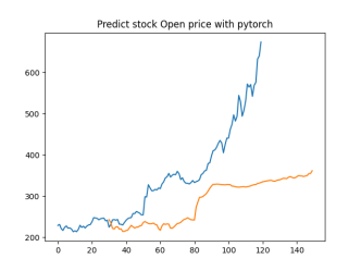
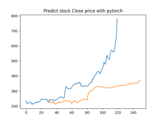
4.4.1. Short-Term Prediction (1 Day)
• The model’s predictions for one day ahead are relatively close to the actual prices, reflecting the market’s immediate behavior.
• Both setups show similar predictions for one-day horizons, indicating that the model effectively captures the immediate trend.
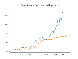
4.4.2. Medium-Term Prediction (5-10 Days)
• The predicted prices over 5 to 10 days begin to show more variation, reflecting short-term market fluctuations.
• The predictions slightly diverge from the current price, as expected, highlighting the challenge of forecasting further into the future.
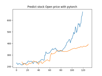
4.4.3. Long-Term Prediction (15-30 Days)
• As the prediction horizon extends to 15, 20, 25, and 30 days, the predicted prices show greater deviation from the starting price.
• These predictions reflect broader market trends and volatility but also indicate potential uncertainties in longer-term forecasts.
The analysis indicates that the model is most reliable for short-term predictions (1 to 5 days), where the predicted stock prices are closer to the actual values. As the prediction horizon extends, accuracy decreases, reflecting the increased uncertainty and complexity of long-term stock price forecasting. This pattern is typical in financial forecasting, where short-term predictions are generally more reliable.
5. Discussion
5.1. Feature Selection
• Impact of Feature Combinations: The results indicate that different combinations of feature columns significantly affect the model’s performance. Specifically, Setup A (using F1-F4: Open, High, Low, Close) and Setup B (using F1-F5: Open, High, Low, Close, Adjusted Close) highlight the importance of including the adjusted close price.
• Role of Adjusted Close Price (F5): Incorporating the adjusted close price (F5) in Setup B provided a more comprehensive view of the stock’s true value by accounting for corporate actions like splits and dividends. While this slightly improved the model’s ability to predict the closing price, it also introduced additional complexity. This complexity might be beneficial for long-term forecasts in some cases but may not significantly contribute to short-term predictions.
• Predictive Power of Basic Trading Metrics: Setup A, which relied solely on basic trading metrics (Open, High, Low, Close), still produced strong results, suggesting that these fundamental price points are highly predictive, particularly for short-term forecasts. This raises the question of whether adding more features always leads to better predictions or if they might introduce unnecessary noise.
5.2. Optimal Time Step
• Finding the Balance: The experiment demonstrated that a 30-day time step offered the optimal balance between capturing relevant information and minimizing noise. A shorter time step (e.g., 20 days) may overlook significant trends, while a longer time step (e.g., 40-60 days) might include extraneous data, thereby weakening the model’s predictive power.
• Time Step and Market Behavior: The 30-day time step aligns well with typical market cycles, where monthly trends are frequently observed in financial data. This indicates that the model effectively utilized these natural cycles to enhance prediction accuracy.
• Generalization Capability: The 30-day time step consistently performed well across different setups, suggesting its robustness across various feature combinations. This time step enabled the model to generalize more effectively, reducing both training and validation losses, which is critical for ensuring the model’s performance on unseen data.
5.3. Time Period Analysis
• Value of Long-Term Data: The 10-year time period proved to be the most effective in both setups, underscoring the importance of using extensive historical data. This extended time span provided the model with a rich dataset that encompassed a wide range of market conditions, from bull markets to bear markets, leading to more accurate predictions.
• Trade-off Between Data Length and Model Complexity: While the 10-year dataset yielded the best performance, it also increased complexity, as the model had to process and learn from a significantly larger dataset. This presents an important consideration: although more data generally enhances accuracy, it also demands more sophisticated models and greater computational resources.
• Capturing Long-Term Trends: Utilizing the full decade of data enabled the model to identify long-term trends and recurring patterns in Tesla’s stock prices, which are crucial for making accurate long-term predictions. However, for more volatile stocks, these long-term trends might be less stable, and the benefits may diminish.
5.4. Prediction Horizon
• Short-Term vs. Long-Term Predictions: The results clearly show that the model was most reliable for short-term predictions (1 to 5 days). This aligns with general market behavior, where short-term trends are easier to predict due to lower volatility and fewer unforeseen events.
• Decreasing Accuracy Over Time: As the prediction horizon extended to 10, 15, 20, 25, and 30 days, the accuracy of the model’s predictions decreased. This trend is expected, as the market becomes more unpredictable over longer periods. For traders and investors, this finding suggests that while LSTM models are useful for short-term trading strategies, caution should be exercised when relying on them for long-term forecasts.
5.5. Model Performance Metrics
• MSE, Train Loss, and Validation Loss: The metrics used to evaluate the model—MSE, train loss, and validation loss—provided a comprehensive view of its performance. In the optimal setups, a low MSE indicated that the model was capable of making accurate predictions, while low train and validation losses suggested that the model did not overfit and could generalize well to new data.
• Consistency Across Setups: The consistent performance metrics across different setups and time periods indicate that the model was robust and stable, which is critical for any predictive model in finance. This reliability is essential for real-world applications and demonstrates the potential for broader adoption of LSTM models in financial markets.
• Insights for Future Research: The analysis of these metrics also highlights areas for future research, such as experimenting with different loss functions or optimization techniques to further improve model performance, particularly for long-term predictions.
6. Conclusion
The Long Short-Term Memory (LSTM) model is advantageous in stock price forecasting due to its ability to handle sequential data through memory units, capturing both short- and long-term trends. It models complex non-linear relationships and accommodates various input features like prices and volume, making it flexible for different financial instruments. LSTM performs well in short-term predictions and scales to large datasets, filtering noise and generalizing better with optimal time step selection. However, LSTM's limitations include sensitivity to hyperparameters, risk of overfitting, interpretability challenges, long training times, reliance on data quality, reduced accuracy in long-term predictions, and limited incorporation of external factors like macroeconomic indicators. Future research could address these issues through automated hyperparameter optimization, advanced regularization techniques, model interpretation tools, accelerated training with better hardware, improved data preprocessing, hybrid models for long-term forecasts, and the integration of external factors and multi-modal data sources to enhance model performance and applicability in financial forecasting.
References
[1]. Selvin, S., Vinayakumar, R., Gopalakrishnan, E. A., Menon, V. K., & Soman, K. P. (2017, September). Stock price prediction using LSTM, RNN and CNN-sliding window model. In 2017 international conference on advances in computing, communications and informatics (icacci) (pp. 1643-1647). IEEE.
[2]. Sunny, M. A. I., Maswood, M. M. S., & Alharbi, A. G. (2020, October). Deep learning-based stock price prediction using LSTM and bi-directional LSTM model. In 2020 2nd novel intelligent and leading emerging sciences conference (NILES) (pp. 87-92). IEEE.
[3]. Jeenanunta, C., Chaysiri, R., & Thong, L. (2018, May). Stock price prediction with long short-term memory recurrent neural network. In 2018 International Conference on Embedded Systems and Intelligent Technology & International Conference on Information and Communication Technology for Embedded Systems (ICESIT-ICICTES) (pp. 1-7). IEEE.
[4]. Srivastava, P., & Mishra, P. K. (2021, October). Stock market prediction using RNN LSTM. In 2021 2nd Global Conference for Advancement in Technology (GCAT) (pp. 1-5). IEEE.
[5]. Wang, Y., Liu, Y., Wang, M., & Liu, R. (2018, October). LSTM model optimization on stock price forecasting. In 2018 17th international symposium on distributed computing and applications for business engineering and science (dcabes) (pp. 173-177). IEEE.
[6]. Patel, J., Patel, M., & Darji, M. (2018). Stock price prediction using RNN and LSTM. Journal of Emerging Technologies and Innovative Research, 5(11), 1069-1079.
[7]. Zhang, X., Gu, N., Chang, J., & Ye, H. (2021). Predicting stock price movement using a DBN-RNN. Applied Artificial Intelligence, 35(12), 876-892.
[8]. Zhao, J., Zeng, D., Liang, S., Kang, H., & Liu, Q. (2021). Prediction model for stock price trend based on recurrent neural network. Journal of Ambient Intelligence and Humanized Computing, 12, 745-753.
Cite this article
Zhang,B. (2025). Stock Price Forecasting Using Long Short-Term Memory Networks: A Comprehensive Analysis of Financial Time-Series Data. Theoretical and Natural Science,87,196-207.
Data availability
The datasets used and/or analyzed during the current study will be available from the authors upon reasonable request.
Disclaimer/Publisher's Note
The statements, opinions and data contained in all publications are solely those of the individual author(s) and contributor(s) and not of EWA Publishing and/or the editor(s). EWA Publishing and/or the editor(s) disclaim responsibility for any injury to people or property resulting from any ideas, methods, instructions or products referred to in the content.
About volume
Volume title: Proceedings of the 4th International Conference on Computing Innovation and Applied Physics
© 2024 by the author(s). Licensee EWA Publishing, Oxford, UK. This article is an open access article distributed under the terms and
conditions of the Creative Commons Attribution (CC BY) license. Authors who
publish this series agree to the following terms:
1. Authors retain copyright and grant the series right of first publication with the work simultaneously licensed under a Creative Commons
Attribution License that allows others to share the work with an acknowledgment of the work's authorship and initial publication in this
series.
2. Authors are able to enter into separate, additional contractual arrangements for the non-exclusive distribution of the series's published
version of the work (e.g., post it to an institutional repository or publish it in a book), with an acknowledgment of its initial
publication in this series.
3. Authors are permitted and encouraged to post their work online (e.g., in institutional repositories or on their website) prior to and
during the submission process, as it can lead to productive exchanges, as well as earlier and greater citation of published work (See
Open access policy for details).
References
[1]. Selvin, S., Vinayakumar, R., Gopalakrishnan, E. A., Menon, V. K., & Soman, K. P. (2017, September). Stock price prediction using LSTM, RNN and CNN-sliding window model. In 2017 international conference on advances in computing, communications and informatics (icacci) (pp. 1643-1647). IEEE.
[2]. Sunny, M. A. I., Maswood, M. M. S., & Alharbi, A. G. (2020, October). Deep learning-based stock price prediction using LSTM and bi-directional LSTM model. In 2020 2nd novel intelligent and leading emerging sciences conference (NILES) (pp. 87-92). IEEE.
[3]. Jeenanunta, C., Chaysiri, R., & Thong, L. (2018, May). Stock price prediction with long short-term memory recurrent neural network. In 2018 International Conference on Embedded Systems and Intelligent Technology & International Conference on Information and Communication Technology for Embedded Systems (ICESIT-ICICTES) (pp. 1-7). IEEE.
[4]. Srivastava, P., & Mishra, P. K. (2021, October). Stock market prediction using RNN LSTM. In 2021 2nd Global Conference for Advancement in Technology (GCAT) (pp. 1-5). IEEE.
[5]. Wang, Y., Liu, Y., Wang, M., & Liu, R. (2018, October). LSTM model optimization on stock price forecasting. In 2018 17th international symposium on distributed computing and applications for business engineering and science (dcabes) (pp. 173-177). IEEE.
[6]. Patel, J., Patel, M., & Darji, M. (2018). Stock price prediction using RNN and LSTM. Journal of Emerging Technologies and Innovative Research, 5(11), 1069-1079.
[7]. Zhang, X., Gu, N., Chang, J., & Ye, H. (2021). Predicting stock price movement using a DBN-RNN. Applied Artificial Intelligence, 35(12), 876-892.
[8]. Zhao, J., Zeng, D., Liang, S., Kang, H., & Liu, Q. (2021). Prediction model for stock price trend based on recurrent neural network. Journal of Ambient Intelligence and Humanized Computing, 12, 745-753.