1. Introduction

The sports industry nowadays is undergoing profound changes in the background of big data. According to the research, over \( 85\% \) of Premier League clubs have established specialized data analysis departments. The collection of game-related data has expanded from traditional basic metrics such as shots and possession rates to cross-domain comprehensive information, including athletes' physical characteristics and social media sentiment. The explosive growth of data has provided innovative possibilities for the construction of prediction models in sports events, while also posing challenges to traditional data analysis methods.

The application of probability and statistical models in sports prediction can be traced back to the mid-20th century with baseball statistics. Bill James revolutionized traditional evaluation methods by using quantitative analysis of player performance. In football, Maher first applied the independent Poisson distribution to predict match scores. Dixon and Coles then improved the accuracy of the model by adding time decay factors and correlation parameters. Karlis and Ntzoufras brought real-time prediction into the spotlight by introducing the Bayesian framework to football game. Today, probability statistical models mainly focus on integrating time-series simulations of random processes and building multi-dimensional prediction models through the combination of diverse data. Probability models combined with advanced technology today can comprehensively analyze the performance of athletes and teams, which has profound significance for promoting event organization and the healthy development of related industries.

The arrangement of the remaining parts of the paper is as follows. In Section 2, the paper introduces the bivariate Poisson distribution model using modified Bessel functions. It estimates parameters of Poisson regression through the EM algorithm and incorporates the concept of a diagonal inflation model to improve the accuracy of draw predictions. Using data from the Italian football league as an example, it compares the accuracy between the simple and bivariate Poisson distribution models in predicting different match scores. As for Section 3, a Bayesian dynamic monitoring model is constructed with the detailed steps for parameter calculation and concepts such as prior and posterior probabilities being explained. The model uses expected calibration error (ECE) and probability ranking scores (RPS) to test calibration and quantify the prediction-actuality consistency respectively. A specific Premier League match is applied to demonstrate the model's real-time win probability outputs. In Section 4, the author focus on the intersection of probability and statistics with other disciplines, briefly discusses the application of combining probability models with machine learning in predicting athlete injuries. And explores the analysis of direction choices by players during penalty shootouts, based on probability and statistics within the framework of game theory. Finally, the concluding remarks are provided in Section 5.

2. Poisson Distribution and Goals Scored Predictions

2.1. Method and Theory

The Poisson distribution is a commonly encountered discrete probability distribution in the fields of statistics and probability, which can be applied to quantify sports competitions. Traditional independent Poisson distribution models usually ignore the correlation between two competing teams for they assume that the scores of them are independent. However, the two-variable Poisson probability framework., by introducing correlation parameters and inflation models, can more accurately reflect the interactive effects in the game and provide a better fit to real-world data. This paper introduces the bivariate Poisson distribution model and its application in football matches [1].

Independent Poisson-distributed random variables \( {X_{i}} (where i=1,2,3) \) have parameters \( {λ_{i}} \) > 0. The variables \( X={X_{1}}+{X_{3}} \) and \( Y={X_{2}}+{X_{3}} \) are jointly distributed as \( BP({λ_{1}},{λ_{2}},{λ_{3}}) \) , with the following joint probability function:

\( {P_{X,Y}}(x,y)=P(X=x,Y=y)={e^{-({λ_{1}}+{λ_{2}}+{λ_{3}})}}\frac{λ_{1}^{x}λ_{2}^{y}}{x!y!}\sum _{i=0}^{min(x,y)}C_{x}^{i}C_{y}^{i}i!{(\frac{{λ_{3}}}{{λ_{1}}{λ_{2}}})^{i}}\ \ \ (1) \)

Defining \( Z=X-Y \) as the difference between two variables, then,

\( PZ=P(X-Y)=P{(X_{1}}-{X_{2}})=z\ \ \ (2) \)

Hence, Z adheres to a Poisson distribution characterized by the parameter \( ({λ_{1}}-{λ_{2}}), \) expressed as \( PD({λ_{1}},{λ_{2}}) \) :

\( {P_{Z}}(z)={e^{-({λ_{1}}-{λ_{2}})}}{(\frac{{λ_{1}}}{{λ_{2}}})^{z/2}}{I_{z}}(2\sqrt[]{{λ_{1}}{λ_{2}}})\ \ \ (3) \)

\( {I_{r}}(x)={(\frac{x}{2})^{r}}\sum _{k=0}^{∞}\frac{{({x^{2}}/4)^{k}}}{k!Γ(r+k+1)}\ \ \ (4) \)

The symbol \( {I_{r}}(x) \) stands for the adjusted Bessel function, which is often applied in engineering, physics, and probability statistics. Specific details are illustrated in the Handbook of Mathematical Functions [2].

Regarding the estimation of parameters, for the \( i-th \) observed value in Poisson regression, the distribution can be obtained as \( ({X_{i}},{Y_{i}})~BP({λ_{1i}},{λ_{2i}},{λ_{3i}}) \) , and \( log({λ_{ki}})={ω_{ki}}{β_{k}} \) when \( k=1,2,3 \) . \( {ω_{ki}} \) as the set of explanatory variables influencing the \( k-th \) parameter, is the vector of explanatory variables. \( {β_{k}} \) represents the degree of influence of the corresponding explanatory variable \( {ω_{ki}} \) on \( log({λ_{ki}}) \) , and is the vector of regression coefficients for the k-th parameter \( {λ_{ki}} \) . Then the EM algorithm can be employed to estimate the parameters The algorithm estimates the latent variables’ expected values based on current parameters in the E(expectation)-step, and updates parameter estimates using the latent variables' expected magnitudes in the M(maximization)-step, maximizing the likelihood function. And the full EM algorithm proceed can be found in Pattern Recognition and Machine Learning [3].

Subsequently, to address the shortcomings of traditional models in predicting draws (e.g., 0-0 or 1-1) and to correct for overdispersion, a diagonal inflated model that founded on the bivariate variables is introduced to make additional adjustments to the probabilities of draws:

\( {P_{D}}(x,y)=\begin{cases} \begin{array}{c} (1-p)BP(x,y|{λ_{1}},{λ_{2}},{λ_{3}} ) ,x≠y \\ (1-p)BP(x,y|({λ_{1}},{λ_{2}},{λ_{3}})+pD(x,θ), x=y \end{array} \end{cases}\ \ \ (5) \)

\( BP(\cdot ) \) is the original bivariate Poisson distribution, describing the case where \( x≠y \) . \( p \) is the inflation proportion parameter which control the adjustment magnitude for the probability of a tie score. \( D(x,θ) \) represents a distribution that is discrete in nature (e.g. Bernoulli distribution) that add additional probability mass when \( x=y \) . In football prediction, J being no greater than three is considered to be adequate.

2.2. Applications

This section primarily discusses the application of the proposed model in football matches. In the bivariate Poisson distribution, \( Z \) which equals to \( X-Y \) measures the variation in the number of goals achieved by the two sides. For each game, the number of goals achieved by the home team and away team are represented by \( {X_{i}} \) and \( {Y_{i}} respectively \) \( and ({X_{i}},{Y_{i}})~BP({λ_{1i}},{λ_{2i}},{λ_{3i}}),i=1,2,⋯,n \) ,

\( log({λ_{1i}})=μ+ho+of{f_{hi}}+de{f_{gi}},log({λ_{2i}})=μ+of{f_{gi}}+de{f_{hi}}\ \ \ (6) \)

Here, \( n \) represents the count of games. The value of \( μ \) does not change and is a fixed parameter while \( ho \) denotes the home team's advantage parameter. Defining \( {h_{i}} \) and \( {g_{i}} \) be the symbols of home team and away team, \( { λ_{1i}},{λ_{2i}} \) are the expectations of goals. Team \( k \) ’s attacking and defensive effectiveness are indicated by \( of{f_{ki }} \) and \( de{f_{ki}} \) . What’s more, the covariance parameter \( {λ_{3}} \) could be summarized through

\( log({λ_{3i}})={β^{con}}+{γ_{1}}β_{hi}^{home}+{γ_{2}}β_{gi}^{away}\ \ \ (7) \)

In this function, \( β_{hi}^{home} \) and \( β_{gi}^{away} \) are contingent on the home the away teams respectively. \( {β^{con}} \) is a fixed parameter. \( {γ_{1}} \) and \( {γ_{2}} \) are parameters take on the values 0 or 1. In case \( ({γ_{1}},{γ_{2}})=(0,0) \) , the constant covariance needs to be considered. The case \( {γ_{1}}=1 \) and \( {γ_{2}}=0 \) illustrate the situation of covariance only determined by the home team, and conversely, it just influenced by the away team.

In defensive leagues, particularly in Serie A (Italian Football League), draws are more common, necessitating the use of a diagonal inflated model. Taking the research results of Dimitris Karlis and Ioannis Ntzoufras as an example. In the regulations of the scoring system during the 1991-1992 Serie A season, the scores awarded for a win and a tie differed by only one point, which directly led to an excessive number of draws. Their experiment result shows that the best-fitting model is a probability model which combined bivariate Poisson distribution with an additional variable specifically introduced to account for the 1-1 situation. By comparing the estimated parameters of the simple Poisson model and the model the paper has constructed, conclusions can be drawn that the simple Poisson model performs well for 0-0 scorelines but underestimates the number of 1-1 results. On the other hand, though the latter model slightly overestimating the frequency of 0-0 scorelines, it accurately predicts the occurrence of 1-1 scorelines [1]. In comparison, the bivariate Poisson model demonstrates superior accuracy. And it is worth to note that as football competition formats continue to evolve, the gap between points awarded for a win and those for a draw has widened, potentially leading to fewer draws in the future. This suggests that more Poisson distribution models may be able to accurately predict match scores in the future.

3. Bayesian Statistics and In-game Win Probability

3.1. Method and Theory

Bayesian statistics is a probability calculation method based on Bayes' theorem. Unlike traditional approaches, which view probability as an objective reflection of long-term frequency, Bayesian methods treat probability as a subjective measure of uncertainty by dynamically updating unknown parameters. This flexible probabilistic framework is particularly well-suited for predicting real-time dynamic win probabilities in sports events. This section will introduce Bayesian statistics and a in-game win probability model for soccer match [4].

Bayes' theorem is defined to update the probability of an event under known conditions:

\( P(A|B)=\frac{P(B|A)P(A)}{P(B)}\ \ \ (8) \)

\( P(A) \) is the prior probability, which represents the subjective belief about event \( A \) before observing the data. \( P(A|B) \) is the posterior probability, which represents the probability of \( A \) occurring after observing data \( B \) . Typically, given the state \( {x_{t}} \) of the random variable \( x \) at time \( t \) , what need to be calculated is the probability that \( x \) equals a certain value from time \( t+1 \) until the final moment of the observation period \( P({x_{ \gt t}}=g|{x_{t}}) \) . Here, \( {x_{ \gt t}} \) is considered following an independent Poisson distribution: \( {x_{ \gt t}}~Pois((T-t)θ) \) . Here, \( θ \) represents the characteristic intensity of the corresponding random variable, which depends on the observed object and the specific calculations will be provided in the application part.

To accurately estimate the posterior distribution of parameters, the Automatic Differentiation Variational Inference (ADVI) algorithm is used to infer Bayesian models. Detailed process can be referred in Automatic Differentiation Variational Inference [5]. Additionally, the Expected Calibration Error (ECE) is introduced to exam the calibration of the model. The probability is divided into 𝑀 intervals to calculate the average deviation between the predicted results and the actual results, determined by the samples’ number in range. Equations derived from that is as follows:

\( ECE=\sum _{m=1}^{M}\frac{|{B_{m}}|}{N}|\bar{y}({B_{m}})-\bar{p}({B_{m}})|\ \ \ (9) \)

\( N \) is the samples’ volume, \( {B_{m}} \) indicates one of the probability intervals defined in the context. The highest likelihood outcome's mean predicted probability is expressed as \( \bar{p}({B_{m}}) \) while \( \bar{y}({B_{M}}) \) represents the proportion of positives in \( {B_{m}} \) . Besides, to evaluate the closeness of the predictions to the actual observed data, the Ranked Probability Score (RPS) is used in the sports game prediction model when \( t \) is the match time [6]:

\( RP{S_{t}}=\frac{1}{2}\sum _{i=1}^{2}{(\sum _{j=1}^{i}{p_{t,j}}-\sum _{j=1}^{i}{e_{j}})^{2}}.\ \ \ (10) \)

In this score, \( \vec{{p_{t}}}=[P(Y=win|{x_{t}}),P(Y=tie|{x_{t}}),P(Y=loss|{x_{t}})] \) are the estimated probabilities at a time frame \( t \) .

3.2. Applications

When constructing a dynamic monitoring model for football game, match state at time \( t \) is given as \( ({x_{t,home}},{x_{t,away}}) \) and the equation (10) can be specified as:

\( P({y_{ \gt t,k}}=g|{x_{t,k}})\ \ \ (11) \)

which reflect the probability of the team \( k \) scoring an additional 𝑔 goals before the final whistle. And the final score of teams \( k \) that is most likely to occur can be predicted as \( {y_{ \lt t,k}}+{y_{ \gt t,k}} \) . Then the goals’ number scored by the team \( k \) after time \( t \) follows the Poisson distribution with parameter \( λ=(T-t){θ_{t,k}} \) . \( {θ_{t}} \) denotes the scoring intensity under time \( t \) and is independent with \( {x_{t}} \) . \( {θ_{t}} \) is a time-varying parameter, the prior estimated strength of the teams is the most important characteristic factor in the early stages of the match, while as the match approaches the end, the team's performance becomes the dominant factor influencing the scoring intensity. It is modeled using a stochastic process:

\( {θ_{t,k}}=inv(\vec{{α_{t}}}×{x_{t,k}}+β+Ho)\ \ \ (12) \)

Here, people define \( {α_{t}} \) as a time-varying regression coefficient which follow a standard normal distribution. \( β \) and \( Ho \) are the intercept and the parameter models the home advantage that both follows the normal distribution \( N(0,2) \) . \( inv \) represents the \( invlogit \) function which is generally a reverse transformation that map the values on the real number range back to the probability interval of 0 to 1.

Determining the current time frame t is a challenge. Some matches have a halftime break at 45 minutes, while others may have additional time added to the first half due to injury stoppages. Therefore, the model chooses to set the time frame for each match to 𝑇=100, where 𝑇=50 represents the halftime. Subsequently, the variables in Table 1 are defined to describe the match state of the teams at each time frame.

Table 1: Three Description Variables

Each variable added has the potential to an exponential expansion of the state space, ensuring that the model accurately captures the likelihood of each team’s goals scored in the remaining match time. During the calibration and estimation process (ECE) of the model, 𝑀 in equation (12) is assigned a value of 5. Table 2 presents the ECEs comparison among the multiple logistic regression model (MLR), logistic regression model (LR) and the random forest (RF) model, with the model constructed in this paper, aggregated for each half and the last 10% of the match. All models were trained under the same feature set get from the top five leagues [7].

Table 2: Comparison Among Four Models’ ECEs

It can be observed that only the proposed model demonstrates a good level of probability calibration. The differences between the models are particular in the final 10% of the match, where the ECE value attained by the proposed model is 0.002 while others’ ECEs remain above 0.1. Among the other three, the RF model performs relatively well while its prediction of the draw probability collapses in the later stages of the match. As for the RPS values, Figure 1 shows that when the game progresses, all prediction models improve as they obtain more information from the match. However, only the Bayesian model steadily delivers accurate predictions by the conclusion of each game.

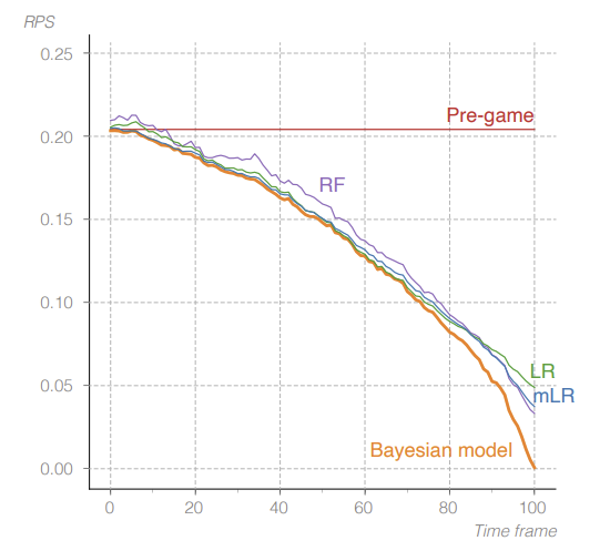
Figure 1: RPS of Four Models [4]

Using the real-time win probability output by the Bayesian model during a match between Queens Park Rangers (QPR) and Manchester City competed on the 2011/12 Premier League campaign as an example. The model results show that Manchester City started the match as the favorites and took control early on, but by the 65th minute of the second half, QPR had taken the lead. Ultimately, Manchester City gave a thrilling comeback during stoppage time [4]. Such real-time win probability models have numerous applications. Firstly, they can enrich audience enjoyment and evaluate gameplay tactics. What’s more, the model's real-time monitoring captures key moments and highlight time during the match, which can be used for post-match analysis and replays. Also, they influence betting outcomes.

4. Interdisciplinary Approaches and Sports Applications

Probabilistic models can not only be used for predicting sports events, but also can be intersect with various disciplines and be applied to diverse areas in sports.

Firstly, probability and statistics can collaborate with machine learning to identify athletes' technical styles or predict injury risks. Taking injury prediction as an example, athletes can use the Functional Movement Screen (FMS) test as an indicator. By completing seven movements like deep squat and hurdle step, participants could obtain different scores. Each movement is scored out of 3 points, where 2 points indicate completing the movement with compensation or assistance, 1 point indicates inability to finish the movement, and 0 points represent there exist pain during the movement. Finally, statistical analysis software such as SPSS is used to analyze the data, and independent sample t-tests are conducted to examine the significance between variables. Result example of Chinese fencers is shown in Table 3 as follows [8].

In training practice, when an athlete's FMS score is \( ≤15 \) , it should draw sufficient attention from the coach. Appropriate corrective exercises and injury prevention practices should be incorporated into the warm-up routine.

Table 3: Injury Probability and FMS Scores of Chinese Fencers [8]

Also, probability and statistics can be integrated with game theory and psychology to analyze the psychological dynamics of athletes in some competitive matches [9]. The most classic example is the Nash equilibrium in penalty shootouts. In each penalty kick, both teams randomly select a goalkeeper and a kicker. The kicker aims to maximize the probability of scoring, while the goalkeeper aims to minimize the opponent's scoring probability. The kicker is free to select the right, left, or center as the target area of the goal, and the goalkeeper can also dive to one of these three directions. It can be defined that when the kicker and goalkeeper choose the same direction, the scoring probability is \( {P_{S}} \) \( ,S=R,L, \) and when they choose opposite directions, the scoring probability is \( {π_{S}} \) . Apparently, \( {π_{S}} \gt {P_{S}} \) and the number \( 1-{π_{S}} \) can be explained with possibility of the ball exiting the field or bouncing off the goalpost. When the goalkeeper jumps to one side, a kick at center could score with probability \( μ \) and the model consider the goalkeeper can usually save a center ball by standing in the center of gate. In summary, the penalty taker and the goalkeeper are engaged in a zero-sum situation, and the strategy space for this game is \( \lbrace Right(R),Center(C),Left(L)\rbrace \) . For details, see Table 4.

Table 4: The Payoff Matrix of Zero-sum Game

Such payoff matrices have different values in different matches, which depend on specific population distribution be denoted as \( dΦ({P_{R}},{P_{L}},{π_{R}},{π_{L}},μ) \) . Then three satisfied assumptions—Assumption Sides and Center (SC), Assumption Sides and Center (SC) and Assumption Kicker’s Side (KS) about scoring probabilities are involved to explain the relationships between the magnitudes of relevant variables in the payoff matrix. The model subsequently explores the characteristic properties of the mixed strategy equilibrium and the predictions that still hold under aggregation in heterogeneous scenarios. A dataset of 459 penalty kicks from the top 5 leagues during the period of 2000 to 2002 is used to test the model's assumptions and predictions. The empirical results align with the model's predictions, demonstrating that such a mixed model is evidently highly useful for tactical planning by teams.

In addition to the aforementioned examples of interdisciplinary applications, probability theory can also be integrated with mechanics to analyze the trajectory of balls in sports events, and with economics to optimize team travel arrangements, among other applications.

5. Conclusion

In this paper, the bivariate Poisson distribution model quantifies the correlation between competing teams, enabling predictions to better align with actual data. The inclusion of the diagonal inflation model addresses the issue of sample overdispersion and improves the accuracy of draw predictions in defensive leagues. Another Bayesian model introduced in this paper for football matches uses several features of each team, treating the number of goals scored as a stochastic process. This model demonstrates good calibration and can analyze player performance during critical moments of a match. The paper also proposes the integrated application of probability and statistics with multiple disciplines, breaking the limitations of single probability models and expanding the direction of probability and statistics applications.

In terms of model improvement, adaptive parameter adjustment mechanisms should be designed for different league styles, such as offensive leagues and defensive leagues, to make score prediction accurately in cross-league scenarios. With regard to future work, the model can also integrate video tracking data (e.g., player heatmaps) and physiological sensor data, using machine learning to deeply extract video features and analyze match outcomes. Additionally, probabilistic statistical models should not only predict data related to the top five leagues but also be applied to evaluate the potential of young players in football academies, establishing long-term tracking databases to broaden the temporal dimension of model applications.

References

[1]. Karlis, D., & Ntzoufras, I. (2003). Analysis of sports data by using bivariate Poisson models. Journal of the Royal Statistical Society: Series D (The Statistician), 52(3), 381–393.
[2]. Abramowitz, M., & Stegun, I. A. (1964). Handbook of mathematical functions (pp. 215–286). Dover Publications.
[3]. Bishop, C. M. (2016). Pattern recognition and machine learning (pp. 423–455). Springer New York.
[4]. Robberechts, P. (2021). A Bayesian approach to in-game win probability in soccer. In Proceedings of the 27th ACM SIGKDD Conference on Knowledge Discovery & Data Mining (pp. 3512–3521). ACM.
[5]. Kucukelbir, A. et al. (2017). Automatic differentiation variational inference. Journal of Machine Learning Research, 18, 1-45
[6]. Gneiting, T., & Raftery, A. E. (2007). Strictly proper scoring rules, prediction, and estimation. Journal of the American Statistical Association, 102(477), 359–378.
[7]. Zhou, L. (2016). A study on the physical motor function and injury probability of outstanding fencing athletes in China. Journal of Capital Institute of Physical Education, 28(4), 344–347.
[8]. Chiappori, P.-A. (2002). Testing mixed-strategy equilibria when players are heterogeneous: The case of penalty kicks in soccer. The American Economic Review, 92(4), 1138–1151.
[9]. Qin, L., & Luo, S. L. (2023). A review of foreign scholars' use of the Bayesian method in the study of sports training and competition. Journal of Guangzhou University of Sport, 43(05), 91-103.
Cite this article
Wang,Y. (2025). Dealing with Probability Statistics Prediction on Sporting Events. Theoretical and Natural Science,100,238-245.
Data availability
The datasets used and/or analyzed during the current study will be available from the authors upon reasonable request.
Disclaimer/Publisher's Note
The statements, opinions and data contained in all publications are solely those of the individual author(s) and contributor(s) and not of EWA Publishing and/or the editor(s). EWA Publishing and/or the editor(s) disclaim responsibility for any injury to people or property resulting from any ideas, methods, instructions or products referred to in the content.
About volume
Volume title: Proceedings of the 3rd International Conference on Mathematical Physics and Computational Simulation
© 2024 by the author(s). Licensee EWA Publishing, Oxford, UK. This article is an open access article distributed under the terms and
conditions of the Creative Commons Attribution (CC BY) license. Authors who
publish this series agree to the following terms:
1. Authors retain copyright and grant the series right of first publication with the work simultaneously licensed under a Creative Commons
Attribution License that allows others to share the work with an acknowledgment of the work's authorship and initial publication in this
series.
2. Authors are able to enter into separate, additional contractual arrangements for the non-exclusive distribution of the series's published
version of the work (e.g., post it to an institutional repository or publish it in a book), with an acknowledgment of its initial
publication in this series.
3. Authors are permitted and encouraged to post their work online (e.g., in institutional repositories or on their website) prior to and
during the submission process, as it can lead to productive exchanges, as well as earlier and greater citation of published work (See
Open access policy for details).