1. Introduction

Quantum information has garnered tremendous interest from physics and mathematics community [1,2]. Evolution of a quantum lattice system is key to understanding nature. Cellular automaton (CA) has long been studied as mathematical model of computation, where a grid of cells evolves according to local rules over discrete time steps [3]. However, classical CA follows local rules that do not incorporate quantum mechanical principles such as superposition, entanglement, and unitary evolution. Quantum cellular automaton (QCA) extends the classical CA framework into the quantum domain, preserving key features like discrete time steps and locality while introducing quantum properties. Quantum cellular automaton (QCA) provides a mathematical framework [4]. The classification of QCAs is a well-posed and exciting question [5]. QCA generalizes classical cellular automata to quantum mechanics, allowing superposition and entanglement while preserving locality and reversibility [6.7]. The concept of QCA is abstract, and using group theory is a good way to understand it [8]. Group theory is the study of algebraic structures called groups, which is used to analyze symmetries in mathematics and physics, and classify structures in algebra [9,10].

Section 2 provides a brief introduction to quantum information and some basic concepts that are important in quantum information, and starts relating QCA. Section 3 introduces the cellular automaton (CA), quantum cellular automaton (QCA), the property of QCA dynamics and Clifford QCA. Section 4 discusses the relation between QCA and group, showing that using group theory to think about QCA is advantageous. Section 5 discusses the applications of QCA in the future.

2. Brief Note on Quantum Information

In quantum information, the trade-off between acquiring information and creating a disturbance

is related to quantum randomness. It is because the outcome of a measurement has a random element that we are unable to infer the initial state of the system from the measurement outcome. Quantum information differs from classical information due to quantum information cannot be copied with perfect fidelity. If we could make a perfect copy of a quantum state, we could measure an observable of the copy without disturbing the original and we could defeat the principle of disturbance. On the other hand, nothing prevents us from copying classical information perfectly. John Bell showed that the predictions of quantum mechanics cannot be reproduced by any local hidden variable theory, and quantum information can be (in fact, typically is) encoded in nonlocal correlations between the different parts of a physical system, correlations with no classical counterpart.

2.1. Hilbert Space (Hermitian Inner Product) Matrix Algebra

In this section, we talk about the inner product and matrix algebra in Hilbert space. Hilbert space connects with many concepts that we would mention later, qubits are represented as vectors in the Hilbert space, quantum gates are unitary operators that act on the state of a qubit in a Hilbert space.

Definition 1. A Hilbert space \( H \) is a complete complex vector space, that is, \( ψ, φ∈H \) and \( a, b∈C \) , then \( aψ+bφ∈H \) .

If \( a, b∈C \) , \( a=[\begin{matrix}{a_{1}} \\ ⋮ \\ {a_{n}} \\ \end{matrix}] \) and \( b=[\begin{matrix}{b_{1}} \\ ⋮ \\ {b_{n}} \\ \end{matrix}] \) and \( v, {v_{1}}, {v_{2}}, w, {w_{1}}, {w_{2}}∈H \) . Then, we have totally 4 properties:

Property 1. \( ⟨av|bw⟩=\overline{a}⟨v|bw⟩=b⟨av|w⟩=\overline{a}b⟨v|w⟩ \)

Property 2. \( ⟨a|b⟩={\overline{a}^{T}}b=\sum _{i=1}^{n}{\overline{a}_{i}}{b_{i}}=[\begin{matrix}{\overline{a}_{1}} & ⋯ & {\overline{a}_{n}} \\ \end{matrix}][\begin{matrix}{b_{1}} \\ ⋮ \\ {b_{n}} \\ \end{matrix}] \)

Property 3. \( ⟨{v_{1}}+{v_{2}}|w⟩=⟨{v_{1}}|w⟩+⟨{v_{2}}|w⟩ \)

Property 4. \( ⟨v|{w_{1}}+{w_{2}}⟩=⟨v|{w_{1}}⟩+⟨v|{w_{2}}⟩ \)

Lemma 2. We define the adjoint of a matrix \( A \) to be \( {A^{*}}={\overline{A}^{T}} \) . It can be verified that for any \( v,w \) in the Hilbert space, we have

\( ⟨v|Aw⟩=⟨{A^{*}}v|w⟩. \)

In fact, this property uniquely determines the adjoint of \( A \) .

Proof. Let \( [\begin{matrix}{v_{1}} \\ ⋮ \\ {v_{n}} \\ \end{matrix}] \) , \( A=[\begin{matrix}{A_{11}} & ⋯ & {A_{1n}} \\ ⋮ & ⋱ & ⋮ \\ {A_{n1}} & ⋯ & {A_{nn}} \\ \end{matrix}] \) and \( w=[\begin{matrix}{w_{1}} \\ ⋮ \\ {w_{n}} \\ \end{matrix}] \) . Then,

\( \begin{matrix}⟨v|Aw⟩ & =[\begin{matrix}{\overline{v}_{1}} & ⋯ & {\overline{v}_{n}} \\ \end{matrix}][\begin{matrix}{A_{11}} & ⋯ & {A_{1n}} \\ ⋮ & ⋱ & ⋮ \\ {A_{n1}} & ⋯ & {A_{nn}} \\ \end{matrix}][\begin{matrix}{w_{1}} \\ ⋮ \\ {w_{n}} \\ \end{matrix}] \\ & ={[{A^{T}}[\begin{matrix}{\overline{v}_{1}} \\ ⋮ \\ {\overline{v}_{n}} \\ \end{matrix}]]^{T}}[\begin{matrix}{w_{1}} \\ ⋮ \\ {w_{n}} \\ \end{matrix}] \\ & ={\overline{[{\overline{A}^{T}}[\begin{matrix}{v_{1}} \\ ⋮ \\ {v_{n}} \\ \end{matrix}]]}^{T}}[\begin{matrix}{w_{1}} \\ ⋮ \\ {w_{n}} \\ \end{matrix}] \\ & =⟨{A^{*}}v|w⟩ \\ \end{matrix} \)

Lemma 3. In a simiar way as Lemma 2, we define a unitary matrix \( U \) , then \( {U^{*}}={U^{-1}} \) , we have

\( ⟨v|Uw⟩=⟨{U^{*}}v|w⟩, \)

because \( {U^{*}}={U^{-1}} \) , we have

\( ⟨v|Uw⟩=⟨{U^{-1}}v|w⟩. \)

2.1.1. Self-Adjoint

Definition 4. The matrix \( A \) is called self-adjoint if \( {A^{*}}=A \) , \( {A^{*}}={(\overline{A})^{T}} \) is called its adjoint.

For example, matrix \( A=[\begin{matrix}1 & i \\ -i & -1 \\ \end{matrix}] \) is self-adjoint, because \( {A^{*}}={[\begin{matrix}1 & -i \\ i & -1 \\ \end{matrix}]^{T}}=[\begin{matrix}1 & i \\ -i & -1 \\ \end{matrix}]=A \) .

2.1.2. Unitary Matrix

Definition 5. The matrix \( U \) is unitary if \( {U^{*}}={U^{-1}} \) or \( U{U^{*}}={U^{*}}U=I \) .

For example, matrix \( U=[\begin{matrix}1 & 0 \\ 0 & i \\ \end{matrix}] \) is a unitary matrix, because \( {U^{*}}=[\begin{matrix}1 & 0 \\ 0 & -i \\ \end{matrix}] \) , then \( U{U^{*}}=[\begin{matrix}1 & 0 \\ 0 & i \\ \end{matrix}][\begin{matrix}1 & 0 \\ 0 & -i \\ \end{matrix}]=[\begin{matrix}1 & 0 \\ 0 & 1 \\ \end{matrix}]=I \) .

2.1.3. Pauli Matrices

Definition 6. The matrices \( {σ_{j}} \) indexed by either \( j∈1,2,3 \) or \( j∈x,y,z \) and defined as

\( X:={σ_{x}}:={σ_{1}}:=[\begin{matrix}0 & 1 \\ 1 & 0 \\ \end{matrix}], Y:={σ_{y}}:={σ_{2}}:=[\begin{matrix}0 & -i \\ i & 0 \\ \end{matrix}], Z:={σ_{z}}:={σ_{3}}:=[\begin{matrix}1 & 0 \\ 0 & -1 \\ \end{matrix}]. \)

are called Pauli matrices. These three Pauli matrices are self-adjoint, and they are unitary matrices.

2.2. Qubit

In this section, we talk about the difference between classical bit and qubit, the general normalized qubit state. The state of a qubit is a vector in the two-dimensional Hilbert space \( {H^{2}} \) . Let we image a coin, a calssical bit is like a coin lying flat on the table, the state is either heads (0) or tails (1). And a qubit is like spinning that coin in the air, when it’s spinning, the state is not just heads (0) or tails (1), it’s a mixture of both until we catch it. This “mixture” is the superposition.

A qubit is a quantum mechanical system described by a two-dimensional Hilbert space denoted by \( H \) and called qubit space. A qubit is a fundamental unit of quantum information, analogous to a classical bit in classical computing. However, unlike a classical bit that can only be in one of two states \( \lbrace 0,1\rbrace \) , a qubit can exist in a superposition of states.

This way each classical bit value is mapped to a qubit state. The smallest nontrivial Hilbert space is two-dimensional. We can denote an orthonormal basis for a two-dimensional vector space as \( \lbrace |0⟩,|1⟩\rbrace \) . However, not every qubit state can be mapped to a classical bit value. This is because the most general normalized qubit state is of the form

\( |ψ⟩=a|0⟩+b|1⟩ \) (1)

with \( a,b∈C \) and \( {|a|^{2}}+{|b|^{2}}=1 \) . Qubit state \( |0⟩ \) corresponds to the classical bit 0, and qubit state \( |1⟩ \) corresponds to the classical bit 1. The superposition case occurs when a qubit exists in a state that is a combination of the basis states \( |0⟩ \) and \( |1⟩ \) , rather than being strictly in one of them, which means \( ab≠0 \) and there is no corresponding classical bit value. The probability of measuring the qubit in the state \( |0⟩ \) is \( {|a|^{2}} \) , the probability of measuring the qubit in the state \( |1⟩ \) is \( {|b|^{2}} \) . After the measurement, the state of qubit collapses to either \( |0⟩ \) or \( |1⟩ \) . The total probability must always equal to 1, so this is also the reason why \( {|a|^{2}}+{|b|^{2}}=1 \) .

Because \( {|a|^{2}}+{|b|^{2}}=1 \) we can find \( α,β,θ∈R \) such that \( a={e^{iα}}cos\frac{θ}{2} \) and \( b={e^{iβ}}sin\frac{θ}{2} \) . Thus, a qubit state has the general form

\( |ψ⟩={e^{iα}}cos\frac{θ}{2}|0⟩+{e^{iβ}}sin\frac{θ}{2}|1⟩. \) (2)

For a 3-dimensional real vector \( a=[\begin{matrix}{a_{1}} \\ {a_{2}} \\ {a_{3}} \\ \end{matrix}] \) , we can define the 2 \( × \) 2 matrix

\( a\cdot σ:=\sum _{j=1}^{3}{a_{j}}{σ_{j}}={a_{1}}{σ_{1}}+{a_{2}}{σ_{2}}+{a_{3}}{σ_{3}}=[\begin{matrix}{a_{3}} & {a_{1}}-i{a_{2}} \\ {a_{1}}+i{a_{2}} & -{a_{3}} \\ \end{matrix}]. \) (3)

The matrix \( a\cdot σ \) is an operation that transform a 3-dimensional real vector \( a=[\begin{matrix}{a_{1}} \\ {a_{2}} \\ {a_{3}} \\ \end{matrix}] \) into a \( 2×2 \) Hermitian matrix using the Pauli matrices \( {σ_{1}} \) , \( {σ_{2}} \) and \( {σ_{3}} \) .

2.3. Tensor Product (between vectors as well as matrices)

In this section, we define a new operation that takes two or more Hilbert spaces to produce a new Hilbert space as their product. Tensor product is significant in building higher dimensional space and representing unitary operators in the following sections.

Let \( {H^{A}} \) and \( {H^{B}} \) be Hilbert spaces, \( |φ⟩∈{H^{A}} \) and \( |ψ⟩∈{H^{B}} \) , then we define

\( |φ⟩⊗|ψ⟩∈{H^{A}}⊗{H^{B}} \) (4)

According to (4), \( |φ⟩⊗|ψ⟩ \) is a vector in the combined Hilbert space \( {H^{A}}⊗{H^{B}} \) . If \( |φ⟩∈{H^{A}} \) and \( |ψ⟩∈{H^{B}} \) and \( a,b∈C \) . Then, we have the following identities.

\( \begin{matrix}(a|φ⟩)⊗|ψ⟩ & =|φ⟩⊗(a|ψ⟩)=a(|φ⟩⊗|ψ⟩) \\ a(|φ⟩⊗|ψ⟩)+b(|φ⟩⊗|ψ⟩) & =(a+b)|φ⟩⊗|ψ⟩ \\ (|{φ_{1}}⟩+|{φ_{2}}⟩)⊗|ψ⟩ & =|{φ_{1}}⟩⊗|ψ⟩+|{φ_{2}}⟩⊗|ψ⟩ \\ |φ⟩⊗(|{ψ_{1}}⟩+|{ψ_{2}}⟩) & =|φ⟩⊗|{ψ_{1}}⟩+|φ⟩⊗|{ψ_{2}}⟩. \\ \end{matrix} \)

In order to simplify the notation, we can also write \( |φ⊗ψ⟩:=|φ⟩⊗|ψ⟩ \) . For vectors \( |{φ_{p}}⟩⊗|{ψ_{p}}⟩∈{H^{A}}⊗{H^{B}} \) with \( p∈\lbrace 1,2\rbrace \) and \( |{φ_{p}}⟩∈{H^{A}} \) , \( |{ψ_{p}}⟩∈{H^{B}} \) we define

\( ⟨{φ_{1}}⊗{ψ_{1}}|{φ_{2}}⊗{ψ_{2}}⟩:=⟨{φ_{1}}|{φ_{2}}{⟩^{{H^{A}}}}⟨{ψ_{1}}|{ψ_{2}}{⟩^{{H^{B}}}}. \) (5)

Lemma 7. Let \( \lbrace |{a_{i}}⟩\rbrace ⊂{H^{A}} \) be an ONB in \( {H^{A}} \) and \( \lbrace |{b_{j}}⟩\rbrace ⊂{H^{B}} \) be an ONB in \( {H^{B}} \) . The set \( \lbrace |{a_{i}}⊗{b_{j}}⟩\rbrace =\lbrace |{a_{i}}⟩⊗|{b_{j}}⟩\rbrace \) forms an ONB in \( {H^{A}}⊗{H^{B}} \) , and for finite-dimensional \( {H^{A}} \) and \( {H^{B}} \) , we have

\( dim({H^{A}}⊗{H^{B}})=dim{H^{A}} dim{H^{B}}. \) (6)

If \( dim{H^{A}}=m \) , and \( dim{H^{B}}=n \) , then let \( |φ⟩=\sum _{i=1}^{m}{c_{i}}|{a_{i}}⟩ \) and \( |ψ⟩=\sum _{j=1}^{n}{d_{j}}|{b_{j}}⟩ \) , \( |{a_{i}}⟩ \) are ONBs in \( {H^{A}} \) and \( |{b_{j}}⟩ \) are ONBs in \( {H^{B}} \) , \( {c_{i}} \) and \( {d_{j}} \) are complex scalars. Thus, the vector in Hilbert space \( {H^{A}}⊗{H^{B}} \) is in the form

\( \begin{matrix}|φ⟩⊗|ψ⟩ & =(\sum _{i=1}^{m}{c_{i}}|{a_{i}}⟩)⊗(\sum _{j=1}^{n}{d_{j}}|{b_{j}}⟩) \\ & =\sum _{i=1}^{m}\sum _{j=1}^{n}{c_{i}}{d_{j}}(|{a_{i}}⟩⊗|{b_{j}}⟩). \\ \end{matrix} \) (7)

Definition 8. In the Hilbert space \( {H^{A}}⊗{H^{B}} \) , the scalar product \( ⟨α|β⟩=\sum _{a,b}^{​}{\overline{α}_{ab}}{β_{ab}} \) , \( α,β∈{H^{A}}⊗{H^{B}} \) is called the tensor product of the Hilbert spaces \( {H^{A}} \) and \( {H^{B}} \) .

If \( {H^{A}}={H^{B}}≅{C^{2}} \) with the ONBs \( \lbrace |{a_{i}}⟩\rbrace =\lbrace |{b_{j}}⟩\rbrace =\lbrace |0⟩,|1⟩\rbrace =\lbrace [\begin{matrix}1 \\ 0 \\ \end{matrix}],[\begin{matrix}0 \\ 1 \\ \end{matrix}]\rbrace \) , where the set \( \lbrace [\begin{matrix}1 \\ 0 \\ \end{matrix}],[\begin{matrix}0 \\ 1 \\ \end{matrix}]\rbrace \) denotes the standard basis in \( {C^{2}} \) . For \( {H^{A}}⊗{H^{B}}≅{C^{4}} \) we have the ONBs \( \lbrace |{a_{i}}⟩⊗|{b_{j}}⟩\rbrace =\lbrace |00⟩,|01⟩,|10⟩,|11⟩\rbrace =\lbrace [\begin{matrix}1 \\ 0 \\ 0 \\ 0 \\ \end{matrix}],[\begin{matrix}0 \\ 1 \\ 0 \\ 0 \\ \end{matrix}],[\begin{matrix}0 \\ 0 \\ 1 \\ 0 \\ \end{matrix}],[\begin{matrix}0 \\ 0 \\ 0 \\ 1 \\ \end{matrix}]\rbrace \) , where the set \( \lbrace [\begin{matrix}1 \\ 0 \\ 0 \\ 0 \\ \end{matrix}],[\begin{matrix}0 \\ 1 \\ 0 \\ 0 \\ \end{matrix}],[\begin{matrix}0 \\ 0 \\ 1 \\ 0 \\ \end{matrix}],[\begin{matrix}0 \\ 0 \\ 0 \\ 1 \\ \end{matrix}]\rbrace \) also denotes the standard basis in \( {C^{4}} \) . Besides, for \( k∈\lbrace 1,2\rbrace \) let \( {a_{k}},{b_{k}}∈C \) and qubit states \( |{φ_{1}}⟩={a_{1}}|0⟩+{b_{1}}|1⟩=[\begin{matrix}{a_{1}} \\ {b_{1}} \\ \end{matrix}], |{φ_{2}}⟩={a_{2}}|0⟩+{b_{2}}|1⟩=[\begin{matrix}{a_{2}} \\ {b_{2}} \\ \end{matrix}] \) . Then, we have

\( \begin{matrix}|{φ_{1}}⟩⊗|{φ_{2}}⟩ & =({a_{1}}|0⟩+{b_{1}}|1⟩)⊗({a_{2}}|0⟩+{b_{2}}|1⟩) \\ & ={a_{1}}{a_{2}}|0⟩⊗|0⟩+{a_{1}}{b_{2}}|0⟩⊗|1⟩+{b_{1}}{a_{2}}|1⟩⊗|0⟩+{b_{1}}{b_{2}}|1⟩⊗|1⟩ \\ & ={a_{1}}{a_{2}}|00⟩+{a_{1}}{b_{2}}|01⟩+{b_{1}}{a_{2}}|10⟩+{b_{1}}{b_{2}}|11⟩ \\ & =[\begin{matrix}{a_{1}}{a_{2}} \\ {a_{1}}{b_{2}} \\ {b_{1}}{a_{2}} \\ {b_{1}}{b_{2}} \\ \end{matrix}], \\ \end{matrix} \) (8)

which represents the state of a two-qubit system.

In a similar way, if \( {H^{C}}≅{C^{2}} \) with the ONB \( \lbrace |0⟩,|1⟩\rbrace \) , then the ONB of \( {H^{A}}⊗{H^{B}}⊗{H^{C}}≅{C^{2}}⊗{C^{2}}⊗{C^{2}}≅{C^{8}} \) is \( \lbrace |000⟩,|001⟩,|010⟩,|011⟩,|100⟩,|101⟩,|110⟩,|111⟩\rbrace \)

\( \begin{matrix}=\lbrace [\begin{matrix}1 \\ 0 \\ 0 \\ 0 \\ 0 \\ 0 \\ 0 \\ 0 \\ \end{matrix}],[\begin{matrix}0 \\ 1 \\ 0 \\ 0 \\ 0 \\ 0 \\ 0 \\ 0 \\ \end{matrix}],[\begin{matrix}0 \\ 0 \\ 1 \\ 0 \\ 0 \\ 0 \\ 0 \\ 0 \\ \end{matrix}],[\begin{matrix}0 \\ 0 \\ 0 \\ 1 \\ 0 \\ 0 \\ 0 \\ 0 \\ \end{matrix}],[\begin{matrix}0 \\ 0 \\ 0 \\ 0 \\ 1 \\ 0 \\ 0 \\ 0 \\ \end{matrix}],[\begin{matrix}0 \\ 0 \\ 0 \\ 0 \\ 0 \\ 1 \\ 0 \\ 0 \\ \end{matrix}],[\begin{matrix}0 \\ 0 \\ 0 \\ 0 \\ 0 \\ 0 \\ 1 \\ 0 \\ \end{matrix}],[\begin{matrix}0 \\ 0 \\ 0 \\ 0 \\ 0 \\ 0 \\ 0 \\ 1 \\ \end{matrix}]\rbrace . \\ \end{matrix} \)

The first notation that includes " \( |⟩ \) " is simple, and the second notation is more complicated.

For the tensor product of dual vectors, we have

\( ⟨φ⊗ψ|=⟨φ|⊗⟨ψ|. \) (9)

The dual ONBs for \( {C^{2}} \) are \( \lbrace ⟨0|,⟨1|\rbrace =\lbrace [\begin{matrix}1 & 0 \\ \end{matrix}],[\begin{matrix}0 & 1 \\ \end{matrix}]\rbrace \) , this set denotes the standard basis in the dual space \( {({C^{2}})^{*}}≅{C^{2}} \) . For \( {C^{4}} \) , dual ONBs are \( \lbrace ⟨00|,⟨01|,⟨10|,⟨11|\rbrace =\lbrace [\begin{matrix}1 & 0 & 0 & 0 \\ \end{matrix}],[\begin{matrix}0 & 1 & 0 & 0 \\ \end{matrix}],[\begin{matrix}0 & 0 & 1 & 0 \\ \end{matrix}],[\begin{matrix}0 & 0 & 0 & 1 \\ \end{matrix}]\rbrace \) , this set denotes the standard basis in the dual space \( {({C^{4}})^{*}}≅{C^{4}} \) . Besides, for \( k∈\lbrace 1,2\rbrace \) , let \( {c_{k}}, {d_{k}}∈C \) , and \( ⟨{ψ_{1}}|={c_{1}}⟨0|+{d_{1}}⟨1|=[\begin{matrix}{c_{1}} & {d_{1}} \\ \end{matrix}] \) , \( ⟨{ψ_{2}}|={c_{2}}⟨0|+{d_{2}}⟨1|=[\begin{matrix}{c_{2}} & {d_{2}} \\ \end{matrix}] \) . In the basis \( \lbrace |{a_{i}}⊗{b_{j}}⟩\rbrace \) , we have

\( \begin{matrix}⟨{ψ_{1}}|⊗⟨{ψ_{2}}| & =({c_{1}}⟨0|+{d_{1}}⟨1|)({c_{2}}⟨0|+{d_{2}}⟨1|) \\ & ={c_{1}}{c_{2}}⟨0|⊗⟨0|+{c_{1}}{d_{2}}⟨0|⊗⟨1|+{d_{1}}{c_{2}}⟨1|⊗⟨0|+{d_{1}}{d_{2}}⟨1|⊗⟨1| \\ & ={c_{1}}{c_{2}}⟨00|+{c_{1}}{d_{2}}⟨01|+{d_{1}}{c_{2}}⟨10|+{d_{1}}{d_{2}}⟨11| \\ & =[\begin{matrix}{c_{1}}{c_{2}} & {c_{1}}{d_{2}} & {d_{1}}{c_{2}} & {d_{1}}{d_{2}} \\ \end{matrix}]. \\ \end{matrix} \) (10)

For \( {C^{8}} \) , dual ONBs are \( \lbrace ⟨000|,⟨001|,⟨010|,⟨100|,⟨011|,⟨101|,⟨110|,⟨111|\rbrace \) . We can find the pattern, either the \( n \) -dimensional space or its dual space has \( n \) standard basis.

2.4. Schmidt Decomposition and Entanglement

In this section, we define a powerful way to express bipartite states, which is Schmidt decomposition, in this way, we can easily determine whether the state is separable or entangled. Also, we use W-state to further explain this powerful tool.

Suppose there are two systems \( A \) and \( B \) , any bipartite state \( |ψ{⟩_{AB}} \) in the Hilbert space \( {H^{A}}⊗{H^{B}} \) can be expressed as the following by Schmidt decomposition:

\( |ψ{⟩_{AB}}=\sum _{k=1}^{r}{λ_{k}}|{u_{k}}{⟩_{A}}⊗|{v_{k}}{⟩_{B}}, \) (11)

where:

• \( \lbrace |{u_{k}}{⟩_{A}}\rbrace \) and \( \lbrace |{v_{k}}{⟩_{B}}\rbrace \) are sets of orthonormal basis vectors in subsystems \( A \) and \( B \) , respectively.

• \( {λ_{k}}≥0 \) are called Schmidt coefficients, satisfying \( \sum _{k}^{​}λ_{k}^{2}=1 \) .

• \( r \) is the Schmidt rank, which is the total number of nonzero Schmidt coefficients.

If the Schmidt rank \( r=1 \) , then the state is separable and can be expressed as \( |ψ⟩={λ_{1}}|{u_{1}}{⟩_{A}}⊗|{v_{1}}{⟩_{B}} \) , in this case, subsystem \( A \) is completely independent of subsystem \( B \) , there is no entanglement. If the Schmidt rank \( r \gt 1 \) , then the state is entangled, the state cannot be written as the tensor product of states in \( {H^{A}} \) and \( {H^{B}} \) .

The W-state for three qubits is

\( |W⟩=\frac{1}{\sqrt[]{3}}(|001⟩+|010⟩+|100⟩), \) (12)

to express this in Schmidt decomposition, we need to divide the system into two subsystems, qubit 1 is one subsystem \( A \) and qubits 2 and 3 form another subsystem \( B \) . Firstly, we can write W-state in another way:

\( |W⟩=\sqrt[]{\frac{1}{3}}(|0{⟩_{A}}⊗|01{⟩_{B}}+|0{⟩_{A}}⊗|10{⟩_{B}}+|1{⟩_{A}}⊗|00{⟩_{B}}), \) (13)

here, the basis for subsystem \( A \) is \( \lbrace |0⟩,|1⟩\rbrace \) , and the basis for subsystem \( B \) is \( \lbrace |00⟩,|01⟩\rbrace ,|10⟩\rbrace ,|11⟩\rbrace \) . Then, we have

\( \begin{matrix}|W⟩ & =\sqrt[]{\frac{1}{3}}(|0{⟩_{A}}⊗(|01{⟩_{B}}+|10{⟩_{B}})+|1{⟩_{A}}⊗|00{⟩_{B}}) \\ & =\sqrt[]{\frac{2}{3}}|0{⟩_{A}}⊗(\frac{1}{\sqrt[]{2}}|01{⟩_{B}}+\frac{1}{\sqrt[]{2}}|10{⟩_{B}})+\sqrt[]{\frac{1}{3}}|1{⟩_{A}}⊗|00{⟩_{B}} \\ & =\sqrt[]{\frac{2}{3}}|0{⟩_{A}}⊗\frac{1}{\sqrt[]{2}}(|01{⟩_{B}}+|10{⟩_{B}})+\sqrt[]{\frac{1}{3}}|1{⟩_{A}}⊗|00{⟩_{B}} \\ & =\sqrt[]{\frac{2}{3}}|0{⟩_{A}}⊗\frac{1}{\sqrt[]{2}}(|01⟩+|10⟩{)_{B}}+\sqrt[]{\frac{1}{3}}|1{⟩_{A}}⊗|00{⟩_{B}}. \\ \end{matrix} \) (14)

The Schmidt rank \( r \) is two, because there are two nonzero Schmidt coefficients. Since the Schmidt rank \( r \gt 1 \) , so the state is entangled between subsystem \( A \) and subsystem \( B \) . The state of subsystem \( A \) is correlated with the state of subsystem \( B \) . If we measure one of subsystems:

1. If we find that subsystem \( A \) is in state \( |0⟩ \) , the state of subsystem \( B \) collapses to \( \frac{1}{\sqrt[]{2}}(|01⟩+|10⟩) \) .

2. If we find that subsystem \( A \) is in state \( |1⟩ \) , the state of subsystem \( B \) collapses to \( |00⟩ \) .

3. If we find that subsystem \( B \) is in state \( \frac{1}{\sqrt[]{2}}(|01⟩+|10⟩) \) , the state of subsystem \( A \) collapses to \( |0⟩ \) .

4. If we find that subsystem \( B \) is in state \( |00⟩ \) , the state of subsystem \( A \) collapses to \( |1⟩ \) .

This dependence shows the quantum correlation between subsystems \( A \) and \( B \) , this correlation is also what we call entanglement between the two subsystems. Entanglement is a relationship involving two or more distinct subsystems. Measurements on subsystem \( A \) can instantaneously affect the outcomes of measurements on subsystem \( B \) , no matter how far apart they are. Without this quantum correlation across subsystems, there would be no entanglement. I think writing states in Schmidt decomposition can beneficially analyze the correlation between subsystems, for example, we can use the qubit in subsystem \( A \) to check the state of subsystem \( B \) is in superposition or not. So I think Schmidt decomposition is a really powerful and helpful tool.

2.5. Finite Depth Quantum Circuit

In this section, we define the quantum gate, the quantum circuit, and the finite depth quantum circuit. A finite depth quantum circuit is like making a multi-layered cake. Each layer of the cake represents a set of quantum gates applied to the qubits, which are like the ingredients on each layer. The total number of layers in the cake corresponds to the finite depth of the circuit, meaning the process stops after a specific number of layers.

In quantum computing, a quantum gate is a fundamental operation that performs a specific transformation on one or more qubits. Unlike many classical logic gates, quantum logic gates are reversible, quantum circuits can perform all operations performed by classical circuits. Quantum gates are unitary operators, and are described as unitary matrices relative to some orthonormal basis. A quantum gate is a unitary operator \( U \) that acts on the state of a qubit or multiple qubits in a Hilbert space. This is how a quantum gate works:

\( |{ψ_{2}}⟩=U|{ψ_{1}}⟩, \) (15)

where \( |{ψ_{1}}⟩ \) is the input quantum state, \( U \) is the unitary matrix which represents the quantum gate, \( |{ψ_{2}}⟩ \) is the resulting quantum state after applying the gate.

Definition 9. A quantum n-gate is a unitary operator \( U:{H^{⊗n}}→{H^{⊗n}} \) . For n = 1, a gate \( U \) is called a unary quantum gate and for n = 2, a gate \( U \) is called a binary quantum gate.

Unary quantum gates are unitary operators \( U:H→H \) , which can be represented in the standard basis \( \lbrace |0⟩,|1⟩\rbrace \) by unitary 2 \( × \) 2 matrices. Most common unary quantum gates include Identity, Pauli-X, Pauli-Y and Pauli-Z.

Binary quantum gates are unitary operators \( U:{H^{⊗2}}→{H^{⊗2}} \) , which can be represented in the standard basis \( \lbrace |00⟩,|01⟩,|10⟩,|11⟩\rbrace \) by unitary 4 \( × \) 4 matrices.

Definition 10. Controlled NOT gate (CNOT) is a quantum gate, CNOT gate operates on a system consisting of 2 qubits. The CNOT gate flips the target qubit if and only if the control qubit is \( |1⟩ \) .

The CNOT gate for control qubit and target qubit in a two-qubit system is a \( 4×4 \) unitary matrix as the following:

Control = Qubit 1, Target = Qubit 2: \( CNO{T_{12}}=[\begin{matrix}1 & 0 & 0 & 0 \\ 0 & 1 & 0 & 0 \\ 0 & 0 & 0 & 1 \\ 0 & 0 & 1 & 0 \\ \end{matrix}], \)

Control = Qubit 2, Target = Qubit 1: \( CNO{T_{21}}=[\begin{matrix}1 & 0 & 0 & 0 \\ 0 & 0 & 0 & 1 \\ 0 & 0 & 1 & 0 \\ 0 & 1 & 0 & 0 \\ \end{matrix}]. \)

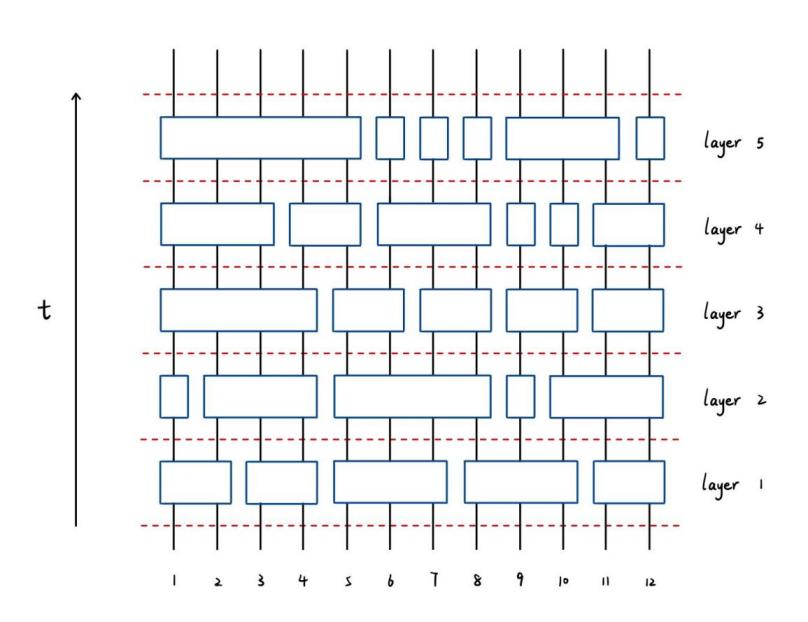
Figure 1: Quantum Circuit Diagram with Twelve Qubits and Five Layers

In a quantum computation, quantum gates are the components of a quantum circuit. A quantum circuit consists of multiple quantum gates applied to qubits. Quantum gates are the tools, while the quantum circuit is the entire mechanism designed to perform a specific quantum computation.

Definition 11. Essentially, a quantum circuit is a framework for using unitary operators (quantum gates) to control and transform the initial quantum state of qubits into a final quantum state, which encodes the result of the quantum computation.

In Figure 1, each vertical line represents a qubit, the blocks represent quantum gates applied to a set of qubits, quantum gates always act on one or more qubits. Each block in a row acts on disjoint sets of qubits, the total number of blocks in the quantum circuit is called its size, and time increases from bottom to top. In the diagram above, there are twelve qubits and five layers.

Definition 12. The depth of a quantum circuit is defined as the number of layers of quantum gates in the quantum circuit diagram.

Definition 13. A finite depth quantum circuit is a quantum circuit with a limited depth required to complete the computation, regardless of the size of quantum circuit or the number of qubits.

Let \( \lbrace {U_{i}}\rbrace \) be a set of unitary operators that act on disjoint sets of qubits within the same layer, then \( {U_{layer}}={U_{1}}⊗{U_{2}}⊗⋯⊗{U_{k}} \) represents the unitary operator for a single layer of the quantum circuit, the tensor product is used because quantum gates in the same layer act on non-overlapping sets of qubits.

Lemma 14. The overall unitary operator for the entire quantum circuit is \( {{U_{circuit}}^{N}}={{U_{l}}^{(1)}}{{U_{l}}^{(2)}}⋯{{U_{l}}^{(N)}} \) , \( N \) is the depth of the quantum circuit.

Proof. According to Definition 11, we let \( |ψ⟩ \) be the initial state of the qubits, then

\( |{ψ_{1}}⟩={{U_{l}}^{(1)}}|ψ⟩ \) (16)

represents the quantum state of the qubits after applying the unitary operator of the first layer, in the similar way, the quantum state of the qubits after applying the first two layers is

\( |{ψ_{2}}⟩={{U_{l}}^{(2)}}|{ψ_{1}}⟩={{U_{l}}^{(2)}}{{U_{l}}^{(1)}}|ψ⟩. \) (17)

So after applying the \( N \) layers in the circuit, the final quantum state of the qubits is

\( \begin{matrix}|{ψ_{final}}⟩ & ={{U_{l}}^{(N)}}{{U_{l}}^{(N-1)}}⋯{{U_{l}}^{(1)}}|ψ⟩ \\ & ={{U_{l}}^{(1)}}{{U_{l}}^{(2)}}⋯{{U_{l}}^{(N)}}|ψ⟩. \\ \end{matrix} \) (18)

Thus, the overall unitary operator for the entire quantum circuit is

\( {{U_{circuit}}^{N}}={{U_{l}}^{(1)}}{{U_{l}}^{(2)}}⋯{{U_{l}}^{(N)}}. \) (19)

3. Clifford Quantum Cellular Automaton

3.1. Quantum Cellular Automaton

A cellular automaton (CA) consists of a regular grid of cells, each in one of a finite number of states. The grid can have any finite number of dimensions (e.g., 1D, 2D, etc.). Every cell has an initial state, and the state of each cell evolves over discrete time steps according to fixed, local rules, all cells in the grid update their states simultaneously at each time step. The new state of each cell depends on its current state and the states of its neighboring cells.

A quantum cellular automaton (QCA) is a lattice-based quantum system where each cell represents a finite-dimensional quantum state. A cell can be in multiple states simultaneously, because of the principle of superposition. The global state of the system evolves in discrete time steps by unitary operators, which ensures the evolution is reversible. The new state of a cell depends on its current state and the states of its neighboring cells.

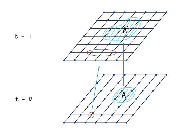
Figure 2: How QCA Works

In Figure 2, the points in the lattice are cells (qubits), \( A \) is the region that contains a set of cells in the lattice at the initial time step (t = 0), the quantum state of this region is the combined state of all qubits within \( A \) at t = 0. \( {A^{ \prime }} \) is the evolved region of \( A \) at t = 1, the quantum state in \( {A^{ \prime }} \) is the result of applying the unitary operator to the quantum state of \( A \) . If there is a matrix associated with every cell or group of cells, then the matrix at t = 0 will be transformed into another matrix at t = 1 under the application of the unitary operator of QCA.

Lemma 15. The QCA dynamics, defined as \( α(A)={U^{*}}AU \) , is a homomorphism, where A is any \( n×n \) matrix and \( U \) is a unitary operator representing the global evolution of the QCA.

Proof. We need to show that \( α \) satisfies preservation of matrix multiplication: \( α(AB)=α(A)α(B) \) , where \( A \) and \( B \) are any \( n×n \) matrices.

Left-Hand Side (LHS):

\( α(AB)={U^{*}}(AB)U, \) (20)

Right-Hand Side (RHS):

\( \begin{matrix}α(A)α(B) & =({U^{*}}AU)({U^{*}}BU) \\ & ={U^{*}}A(U{U^{*}})BU \\ & ={U^{*}}ABU. \\ \end{matrix} \) (21)

So LHS is equal to RHS, which means that \( α \) preserves matrix multiplication. In conclusion, the QCA dynamics \( α(A)={U^{*}}AU \) is a homomorphism.

Any \( 2×2 \) matrix can be written as \( {a_{1}}I+{a_{2}}X+{a_{3}}Y+{a_{4}}Z \) , \( {a_{1}},{a_{2}},{a_{3}},{a_{4}}∈C \) , and \( I \) is the identity matrix, \( X, Y, Z \) are Pauli matrices as mentioned in Definition 6. We denote the dynamics of a QCA by \( α:A→α(A) \) , \( A \) is any matrix and \( α \) is linear transformation, which maps a matrix \( {a_{1}}I+{a_{2}}X+{a_{3}}Y+{a_{4}}Z \) to a new matrix \( {a_{1}}α(I)+{a_{2}}α(X)+{a_{3}}α(Y)+{a_{4}}α(Z) \) . We know that \( α(I)=I \) , if we can figure out where \( α \) maps \( X \) , \( Y \) and \( Z \) to, then we can figure out where \( α \) maps all the matrices to. Actually, we just need to know \( α(X) \) and \( α(Z) \) , because \( Y=[\begin{matrix}0 & -i \\ i & 0 \\ \end{matrix}]=iXZ \) and because of Lemma 15, then \( α(Y)=iα(X)α(Z) \) . So if we know \( α(X) \) and \( α(Z) \) , then we know \( α(Y) \) . Thus, if we know \( α(X) \) and \( α(Z) \) , then we know what the new matrix \( {a_{1}}α(I)+{a_{2}}α(X)+{a_{3}}α(Y)+{a_{4}}α(Z) \) exactly is. To relate to Section 2.5, quantum circuit is a special class of QCA, but not all QCA comes from quantum circuits. In the QCA dynamics \( α(A)={U^{*}}AU \) , if \( U \) is the overall unitary operator of the quantum circuit, then this QCA comes from quantum circuit.

3.2. Clifford Quantum Cellular Automaton

Definition 16. A Clifford Quantum Cellular Automaton (Clifford QCA) is a specific type of Quantum Cellular Automaton (QCA). This evolution of system is controlled by a global unitary operator \( U \) , constructed by local Clifford gates, ensuring locality. And the system is reversible, the state of the system at any previous time step can be uniquely determined from its state at a later time step. Let \( {P_{n}} \) be the Pauli group on n-qubits, consisting of all tensor products of Pauli operators \( \lbrace I,X,Y,Z\rbrace \) with phase factors \( ±1 \) , \( ±i \) . For Clifford QCA,

\( α(P)={U^{*}}PU∈{P_{n}}, ∀P∈{P_{n}}, \)

where \( U \) is the global unitary operator. This means that for any Pauli operator \( P \) , its image \( α(P) \) is also a Pauli operator.

4. Results

4.1. QCA and Automorphism

Definition 17. An automorphism of a group \( G \) is an isomorphism from \( G \) to itself. If \( f \) is the function such that:

1. \( f:G→G \) .

2. \( f(x*y)=f(x)*f(y) \) .

3. \( f \) is bijective.

Theorem 18. The conjugation by an invertible matrix is an automorphism.

Proof. Let \( {M_{n}}(F) \) be the group that contains \( n×n \) matrices over the field \( F \) . And let \( B \) be an \( n×n \) invertible matrix, \( A \) is any \( n×n \) matrix, then we define the map: \( {φ_{B}}(A)=BA{B^{-1}} \) . If this map satisfy the following, then it is an automorphism:

1. \( {φ_{B}}:{M_{n}}(F)→{M_{n}}(F) \) .

2. \( { φ_{B}}(AC)={φ_{B}}(A){φ_{B}}(C) \) , where \( C \) is any \( n×n \) matrix.

3. \( {φ_{B}} \) is bijective.

5. To prove \( {φ_{B}}:{M_{n}}(F)→{M_{n}}(F) \) : We know that \( A \) is an \( n×n \) matrix, B is an \( n×n \) invertible matrix, and \( {B^{-1}} \) is also an \( n×n \) invertible matrix, so the product \( BA{B^{-1}} \) is also an n by n matrix. \( A∈{M_{n}}(F) \) , and \( BA{B^{-1}}∈{M_{n}}(F) \) , so the map \( {φ_{B}}(A)=BA{B^{-1}} \) satisfies \( {φ_{B}}:{M_{n}}(F)→{M_{n}}(F) \) .

6. To prove \( {φ_{B}}(AC)={φ_{B}}(A){φ_{B}}(C) \) , where \( C \) is any \( n×n \) matrix:Left-Hand Side (LHS):

\( {φ_{B}}(AC)=BAC{B^{-1}}, \) (22)

Right-Hand Side (RHS):

\( \begin{matrix}{φ_{B}}(A){φ_{B}}(C) & =(BA{B^{-1}})(BC{B^{-1}}) \\ & =BA({B^{-1}}B)C{B^{-1}} \\ & =BAC{B^{-1}}. \\ \end{matrix} \) (23)

So LHS is equal to RHS, which means that \( {φ_{B}}(AC)={φ_{B}}(A){φ_{B}}(C) \) .

7. To prove that \( {φ_{B}} \) is bijective, we need to show

• Injectivity: If \( {φ_{B}}(A)={φ_{B}}(C) \) , then \( A=C \) .

Suppose \( BA{B^{-1}}=BC{B^{-1}} \) , then multiplying both sides with \( {B^{-1}} \) on the left and \( B \) on the right:

\( \begin{matrix}{B^{-1}}(BA{B^{-1}})B & ={B^{-1}}(BC{B^{-1}})B \\ A & =C. \\ \end{matrix} \) (24)

So \( {φ_{B}} \) is injective.

• Surjectivity: Given any matrix D, we need to find some A such that \( {φ_{B}}(A)=D \) , i.e.,

\( \begin{matrix}BA{B^{-1}} & =D \\ A & ={B^{-1}}DB. \\ \end{matrix} \) (25)

Since A exists for any D, so \( {φ_{B}} \) is surjective.

Thus, \( {φ_{B}} \) is bijective.

In conclusion, the map \( {φ_{B}} \) is an automorphism, so the conjugation by an invertible matrix is an automorphism.

Lemma 19. Quantum cellular automaton is an automorphism.

Proof. According to Lemma 15, we know that the QCA dynamics \( α(A)={U^{*}}AU \) is a homomorphism, where A is any \( n×n \) matrix, and \( U \) is an \( n×n \) unitary operator. We only need to prove that \( α(A):{M_{n}}(F)→{M_{n}}(F) \) and \( α(A) \) is bijective.

8. The mapping preserves the space: \( A \) is an \( n×n \) matrix, \( U \) is an \( n×n \) unitary matrix, \( {U^{*}} \) is also an \( n×n \) unitary matrix, so \( {U^{*}}AU \) is an \( n×n \) matrix. \( A∈{M_{n}}(F) \) and \( {U^{*}}AU∈{M_{n}}(F) \) , so \( α(A):{M_{n}}(F)→{M_{n}}(F) \) , which means \( α(A) \) preserves the space.

9. The mapping is bijective: Since \( U \) is unitary, we define the inverse of \( α \) as \( {α^{-1}}(A)=UA{U^{*}} \) . Then, we need to check \( {α^{-1}} \) is indeed the inverse:

\( \begin{matrix}{α^{-1}}(α(A)) & =U({U^{*}}AU){U^{*}} \\ & =A. \\ α({α^{-1}}(A)) & ={U^{*}}(UA{U^{*}})U \\ & =A. \\ \end{matrix} \) (26)

Thus, \( α \) is bijective. So QCA is an automorphism.

4.2. Conjugation by a Quantum Circuit

Theorem 20. The conjugation by a (finite depth) quantum circuit is a quantum cellular automaton.

Proof. Let \( U \) be a unitary matrix, which represents a quantum circuit, and \( A \) be a local operator. So we define the conjugation by a quantum circuit as \( φ(A):A→UA{U^{-1}}=UA{U^{*}} \) . We suppose that \( A \) is supported in region \( X \) , which means that \( A \) only acts on qubits nontrivially within \( X \) , and \( A \) acts as the identity outside of \( X \) . If \( Y \) is disjoint from \( X \) , then \( A \) commutes with any operator supported in \( Y \) . Firstly, we only focus on the case when \( U \) is a single-layer circuit. We assume that \( U=\prod _{γ}^{​}{G_{γ}} \) , where \( {G_{γ}} \) represents the quantum gate in quantum circuit, there are finite many \( {G_{γ}} \) intersect with \( A \) , and the others don’t intersect with \( A \) , so all \( {G_{γ}} \) commute with \( A \) except finitely many \( {G_{γ}} \) that intersect with \( A \) . Let the support of \( {G_{γ}} \) be \( Z \) , so we have

\( \begin{matrix}UA{U^{*}} & =\prod _{γ}{G_{γ}} A  (\prod _{γ}{G_{γ}}{)^{*}} \\ & =\prod _{γ}{G_{γ}} A  \prod _{γ}G_{γ}^{*} \\ & =\prod _{Z∩X≠∅}^{​}{G_{γ}}A \prod _{Z∩X≠∅}^{​}G_{γ}^{*}. \\ \end{matrix} \) (27)

The support of \( UA{U^{*}} \) is the union of \( X \) and the support of all \( {G_{γ}} \) that intersect with \( A \) . And we assume that the support of \( {G_{γ}} \) has bounded diameter that is less than \( r \) , so for \( {G_{γ}} \) that intersect with \( A \) , the farthest distance between the boundary of X and the point on the support of \( {G_{γ}} \) is less than the bounded diameter of support of \( {G_{γ}} \) , which is also less than \( r \) . So \( UA{U^{*}} \) is supported within \( {B_{r}}(X)=\lbrace y is the point | d(y,X) \lt r\rbrace \) .

Then, in a similar way, when \( U \) has multiple layers, then the region where \( UA{U^{*}} \) is supported expands with each layer, after \( n \) layers, the \( UA{U^{*}} \) is supported within a neighborhood of \( X \) that is a ball of radius \( nr \) , denoted as \( {B_{nr}}(X)=\lbrace z is the point | d(z,X) \lt nr\rbrace \) , where \( r \) represents the quantity of expansion of region per layer.

All in all, \( A \) is supported in region \( X \) , then \( UA{U^{*}} \) is supported in region \( {B_{nr}}(X) \) , and \( {B_{nr}}(X) \) always contains \( X \) , which means that \( UA{U^{*}} \) is supported in a neighborhood of \( X \) . Thus, the conjugation by (finite depth) quantum circuit is locality-preserving, so the conjugation by a (finite depth) quantum circuit is a quantum cellular automaton.

If the operation of a QCA can be decomposed into the operations of several local quantum circuits, then this QCA can be written as the conjugation by the quantum circuits, so not all QCAs are the conjugation by the quantum circuit.

\( SWAP \) is a quantum gate, swap gate swaps two qubits: \( |00⟩→|00⟩ \) , \( |01⟩→|10⟩ \) , \( |10⟩→|01⟩ \) , \( |11⟩→|11⟩ \) . Swap gate can be represented by a unitary matrix \( SWAP=[\begin{matrix}1 & 0 & 0 & 0 \\ 0 & 0 & 1 & 0 \\ 0 & 1 & 0 & 0 \\ 0 & 0 & 0 & 1 \\ \end{matrix}] \) . According to Definition 10, we have \( SWAP=CNO{T_{12}} CNO{T_{21}} CNO{T_{12}} \) , \( CNO{T_{12}} \) and \( CNO{T_{21}} \) are unitary matrices, and \( CNOT \) is a quantum gate, \( SWAP \) can be written as the product of three quantum gates, so \( SWAP \) is a quantum circuit.

Lemma 21. \( SWAP \) is the conjugation by a quantum circuit.

Proof. By the definition, \( SWAP:U⊗V→V⊗U \) , where \( U \) and \( V \) are two operators. If we prove that \( SWAP:U⊗V→C(U⊗V){C^{*}} \) , where \( C \) is a quantum circuit, and \( C(U⊗V){C^{*}}=V⊗U \) , then \( SWAP \) is the conjugation by a quantum circuit. We know that \( SWAP \) can be represented as a unitary matrix, we find that \( SWA{P^{*}}=SWAP \) . We establish that \( C=SWAP \) , so \( C(U⊗V){C^{*}}=SWAP(U⊗V)SWA{P^{*}}=SWAP(U⊗V)SWAP=V⊗U \) , so \( SWAP \) is the conjugation by a quantum circuit.

4.3. QC is a Subgroup of QCA

Proposition 22. \( QC⊊QCA \) , where \( QC \) represents the set of conjugations by the quantum circuits, \( QCA \) represents the set of QCAs. Besides, \( QC \) is a subgroup of \( QCA \) , denoted as \( QC≤QCA \) .

Proof. According to Lemma 19, the set of QCAs is the set of automorphisms, which forms a group under composition, so the set of QCAs is a group. As we mentioned before, some QCAs can be decomposed by into several local quantum circuits, but some QCAs cannot, so \( QC⊊QCA \) . And let \( B \) be an \( n×n \) unitary matrix, and \( A \) is any \( n×n \) matrix, so the conjugation by a quantum circuit is denoted as \( {φ_{B}}(A)=BA{B^{-1}} \) , the inverse of this is \( φ_{B}^{-1}(A)={B^{-1}}AB \) , because \( B \) is an \( n×n \) unitary matrix, so the set of conjugations by the quantum circuits is closed under inverse. And let \( {φ_{M}}(A)=MA{M^{-1}} \) , \( {φ_{N}}(A)=NA{N^{-1}} \) be the elements in the set of conjugations by the quantum circuits, where \( M \) and \( N \) are \( n×n \) unitary matrices, and \( A \) is any \( n×n \) matrix. \( {φ_{N}}({φ_{M}}(A))=NMA{M^{-1}}{N^{-1}}=(NM)A{(NM)^{-1}} \) , since the matrix \( NM \) is an \( n×n \) unitary matrix, so the set of conjugations by the quantum circuits is closed under multiplication. Thus, the set of conjugations by the quantum circuits is a subgroup of set of QCAs, denoted as \( QC≤QCA \) .

4.4. QC is a Normal Subgroup of QCA

Proposition 23. \( QC \) is a normal subgroup of \( QCA \) , denoted as \( QC⊴QCA \) , where \( QC \) represents the set of conjugations by the quantum circuits and \( QCA \) represents the set of QCAs.

Proof. Let \( α \) be a QCA, \( β \) be the conjugation by quantum circuit. We need to prove that \( αβ{α^{-1}}∈QC \) , which means that \( αβ{α^{-1}} \) is the conjugation by quantum circuit. Suppose \( β(A)=BA{B^{-1}} \) , where \( B \) is an \( n×n \) unitary matrix that represents the quantum circuit, \( A \) is any \( n×n \) matrix, \( O \) is the matrix on qubits. We have

\( αβ{α^{-1}}(O)=α(B{α^{-1}}(O){B^{-1}}), \) (28)

because of Lemma 19, we have

\( \begin{matrix}αβ{α^{-1}}(O) & =α(B)α({α^{-1}}(O))α({B^{-1}}) \\ & =α(B)Oα({B^{-1}}), \\ \end{matrix} \) (29)

because of Lemma 19, so \( α({B^{-1}})=α{(B)^{-1}} \) , so

\( αβ{α^{-1}}(O)=α(B)Oα{(B)^{-1}}. \) (30)

We know that \( n×n \) unitary matrix \( B \) represents the quantum circuit, \( α \) operates on a quantum circuit \( B \) , meaning that \( α \) operates on every quantum gate in circuit, in each layer, quantum gates will act on more qubits, the number of qubits every gate acts on is limited. So \( α(B) \) is also a quantum circuit, but the number of qubits that each quantum gate acts on has increased. We find that \( αβ{α^{-1}}(O)=α(B)Oα{(B)^{-1}} \) , where \( α(B) \) is a quantum circuit and \( O \) is the matrix on qubits, so \( α(B)Oα{(B)^{-1}} \) is the conjugation by the quantum circuit, so \( QC \) is a normal subgroup of \( QCA \) , denoted as \( QC⊴QCA \) , where \( QC \) represents the set of conjugations by the quantum circuits and \( QCA \) represents the set of QCAs.

4.5. QCA/QC is an Abelian Group

Definition 24. The group G is abelian if \( x*y=y*x \) for all \( x,y∈G \) .

Proposition 25. \( QCA/QC \) is an abelian group, where \( QCA \) represents the set of QCAs, and \( QC \) represents the set of conjugations by the quantum circuits.

Proof. Suppose \( α,β∈QCA \) , according to Proposition 23, we have \( QCA/QC=\lbrace εQC | ε∈QCA\rbrace \) . We suppose that two elements in this group are \( αQC \) and \( βQC \) , to show that \( QCA/QC \) is an abelian group, we need to show that \( (αQC)(βQC)=(βQC)(αQC) \) , equivalent to showing that \( (αβ)QC=(βα)QC \) , which means that we need to show that \( αβ=AβBαC≃βα \) , where \( A,B,C∈QC \) . According to Lemma 21, we have \( SWAP∈QC \) .

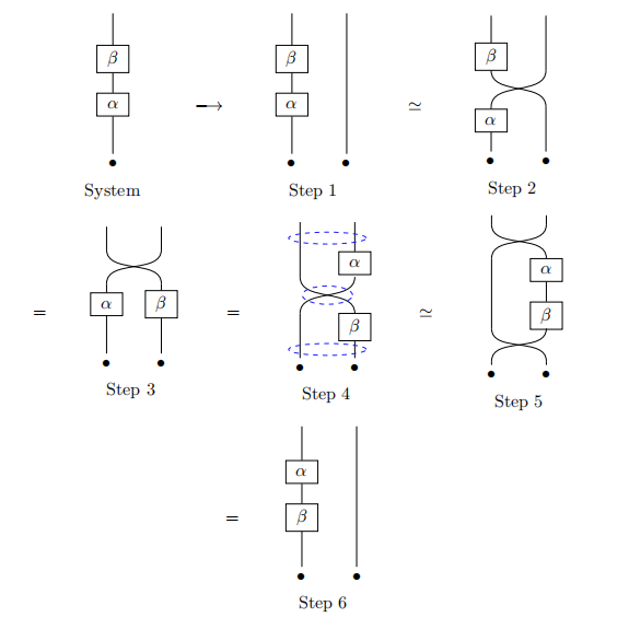
Figure 3: The Operations on a System

In Figure 3, the points represent qubits, and \( α \) acts on qubit first and \( β \) acts on qubit secondly, then we have a system. Next, we do the stabilization on this system, meaning that the original system does the tensor product with another system that only contains identity operators. Then, though elements in the new whole system have one more dimension, they are essentially unchanged, as shown in Step 1. Subsequently, we insert a \( SWAP \) in Step 2, the new system is equal to the system shown in Step 3, which is also equal to the system shown in Step 4. Then, we insert three \( SWAP \) in three places circled with dashed line, then we get the system in Step 5, which is equal to the system shown in Step 6. The following is the process we do in Figure 3:

\( \begin{matrix}β∘α & \vec{Stabilization} & (β ⨂ I)∘(α ⨂ I) & ⋯⋯ & Step 1 \\ & & ≅(β ⨂ I)∘SWAP∘(α ⨂ I) & ⋯⋯ & Step 2 \\ & & =SWAP∘(I ⨂ β)∘(α ⨂ I) & ⋯⋯ & Step 3 \\ & & =SWAP∘(α ⨂ I)∘(I ⨂ β) & & \\ & & =(I ⨂ α)∘SWAP∘(I ⨂ β) & ⋯⋯ & Step 4 \\ & & =SWAP∘(I ⨂ α)∘(I ⨂ β)∘SWAP & ⋯⋯ & Step 5 \\ & & =(α ⨂ I)∘(β ⨂ I) & ⋯⋯ & Step 6 \\ \end{matrix} \) (31)

We can see that the order of \( α \) and \( β \) is reversed in the first subsystem in step 6 compared to step 1, and only identity operators act on the second subsystem where we do stabilization. Thus, we find that \( (β⊗I)∘(α⊗I) \) is equivalent to \( (α⊗I)∘(β⊗I) \) by applying \( SWAP \) operations, \( A,B,C∈QC \) , they are \( SWAP \) operations here, so \( αβ=AβBαC≃βα \) , then \( QCA/QC \) is an abelian group.

5. Discussion

Our study explores QCA through group theory, offering new insights into its mathematical structure. While QCA has primarily been studied in the context of quantum computing and quantum information, its broader applications remain largely unexplored. One intriguing direction is whether QCA can be used as a computational tool to solve hard problems in group theory. Since group-theoretic methods help analyze QCA dynamics, it is natural to ask the reverse — can QCA provide novel solutions for problems like finite simple group classification or infinite group representations? If so, it could introduce new approaches to approach these problems that might be faster or more effective than classical methods. Future research should focus on establishing a formal connection between QCA models and algebraic structures, possibly leading to novel quantum algorithms that extend beyond conventional quantum algorithms.

References

[1]. Gregg Jaeger. Quantum information. Springer, 2007.
[2]. Wolfgang Scherer. Mathematics of quantum computing. Vol. 11. Springer, 2019.
[3]. Edgar F Codd. Cellular automata. Academic press, 2014.
[4]. Terry Farrelly. “A review of quantum cellular automata”. In: Quantum 4 (2020), p. 368.
[5]. Michael Freedman and Matthew B Hastings. “Classification of quantum cellular automata”. In: Communications in Mathematical Physics 376 (2020), pp. 1171–1222.
[6]. Bei Zeng, Xie Chen, Duan-Lu Zhou, Xiao-Gang Wen, et al. Quantum information meets quantum matter. Springer, 2019.
[7]. Benjamin Schumacher and Reinhard F Werner. “Reversible quantum cellular automata”. In: arXiv preprint quant-ph/0405174 (2004).
[8]. Jeongwan Haah. “Clifford quantum cellular automata: Trivial group in 2D and Witt group in 3D”. In: Journal of Mathematical Physics 62.9 (2021).
[9]. John F Humphreys. A course in group theory. Vol. 6. OUP Oxford, 1996.
[10]. William Raymond Scott. Group theory. Courier Corporation, 2012.
Cite this article
Bai,R. (2025). Quantum Cellular Automata and Groups. Theoretical and Natural Science,92,178-193.
Data availability
The datasets used and/or analyzed during the current study will be available from the authors upon reasonable request.
Disclaimer/Publisher's Note
The statements, opinions and data contained in all publications are solely those of the individual author(s) and contributor(s) and not of EWA Publishing and/or the editor(s). EWA Publishing and/or the editor(s) disclaim responsibility for any injury to people or property resulting from any ideas, methods, instructions or products referred to in the content.
About volume
Volume title: Proceedings of the 3rd International Conference on Mathematical Physics and Computational Simulation
© 2024 by the author(s). Licensee EWA Publishing, Oxford, UK. This article is an open access article distributed under the terms and
conditions of the Creative Commons Attribution (CC BY) license. Authors who
publish this series agree to the following terms:
1. Authors retain copyright and grant the series right of first publication with the work simultaneously licensed under a Creative Commons
Attribution License that allows others to share the work with an acknowledgment of the work's authorship and initial publication in this
series.
2. Authors are able to enter into separate, additional contractual arrangements for the non-exclusive distribution of the series's published
version of the work (e.g., post it to an institutional repository or publish it in a book), with an acknowledgment of its initial
publication in this series.
3. Authors are permitted and encouraged to post their work online (e.g., in institutional repositories or on their website) prior to and
during the submission process, as it can lead to productive exchanges, as well as earlier and greater citation of published work (See
Open access policy for details).