1. Introduction

In modern society, where a house usually acts as one of the most significant investments made by people, the housing market plays a pivotal role in shaping both individual wealth and indicating financial stability [1]. Therefore, it is important to examine the factors influencing housing prices for both buyers and policymakers. As the state whose GDP comprises the biggest proportion of the GDP in the United States, the housing price in California is influenced by a complex interplay of different factors [2]. Therefore, the purpose of the essay is to examine the factors influencing housing prices in California, which can help people to obtain a perspective to observe the US economy.

Housing prices can be predicted using multiple methods according to different conditions. Lim et al. compared the accuracy of artificial neural networks (ANN), autoregressive integrated moving average (A, and multiple regression analysis (MRA) in predicting Singapore condominium prices and discovered that the ANN model can reach high precision in multiple ways [3]. Also, focusing on the differences between the ANN and the MRA models, Nguyen and Cripps concluded that the ANN performs better than the MRA when using a moderate to large sample size [4]. Truong et al. explored different models in machine learning for predicting house prices using the Beijing house price dataset and found out that the error occurs the least in the Random Forest method, in spite of overfitting problems [5].

The specific method of linear regression can be applied in multiple ways. Fedotova et al. described a study of the application of MRL in software development estimation and showed that the test using the MRL model provided better estimations than judgements made by the expert [6]. Furthermore, Zhang combined it with the Spearman correlation coefficient in the dataset of Boston housing prices and proved its effectiveness [7]. Moreover, Thamarai and Malarvizhi suggested that the multiple linear regression method outperformed decision tree regression in predicting house prices [8].

2. Methods

2.1. Data source

The dataset utilized in this study was obtained from the Kaggle website (California House Price). The sample data was collected by Shibu Mohapatra from the US Census Bureau, containing 20640 groups of data of blocks in California in total. The dataset was originally in .csv format.

2.2. Variable selection

After examining the data, 207 samples were found to contain null values, hence, the analysis was conducted on the remaining 20433 samples after the removal of the null values. In this paper, eight independent variables (longitude, latitude, housing_median_age, total_rooms, total_bedrooms, population, households, median_income) and one dependent variable (house_median_value) are selected from the dataset, as shown in Table 1:

Table 1: List of variables

2.3. Method introduction

This study employs multiple linear regression to analyse the potential factors influencing housing prices and their correlations, along with preliminary correlation analysis. Linear regression is a statistical analysis method that utilizes regression analysis to determine the quantitively dependent relationship between two or more variables [9, 10]. The relationship between the independent and dependent variables can be approximated by a straight line. The situation where two or more independent variables are involved is called multiple linear regression. It can be described by the formula:

\( y={β_{0}}+{β_{1}}{x_{1}}+{β_{2}}{x_{2}}+⋯+{β_{p}}{x_{p}}+ε \) (1)

In this formula, β₀​ is the intercept, representing the expected value of y when all independent variables are zero, and \( ε \) accounts for the variability in y that the model does not explain. Moreover, \( {β_{1}}, {β_{2}},… {β_{p}} \) are the regression coefficients, each measuring the effect of a one-unit increase in the corresponding independent variable x_i.

Furthermore, the issue of multicollinearity will be examined by using the variance inflation factor (VIF), which measures the increase in the variance of an estimated regression coefficient due to collinearity.

3. Results and discussion

3.1. Descriptive analysis

In order to evaluate the potential of various independent variables to predict housing prices, correlation analyses are performed to determine the relationships between variables preliminarily.

First, scatter plots were generated to visually test the linear relationship between each independent and the dependent variable. Among the variables tested, x8 showed the most significant positive linear correlation with housing prices. Figure 1 indicates that housing prices tend to rise as median income increases.

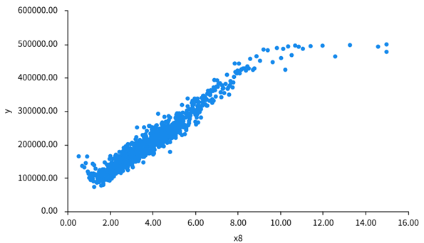
Figure 1: Scatter plot of x8 and y

This figure suggests that median income is a key factor in predicting housing prices in California, as higher-income areas typically correlate with higher property values.

In contrast, the scatter plots for other independent variables suggest weaker or no apparent relationship with housing prices. For example, Figure 2 exhibits a clustered distribution with no apparent trend, indicating that the geographical position of a California block has little effect on its housing price.

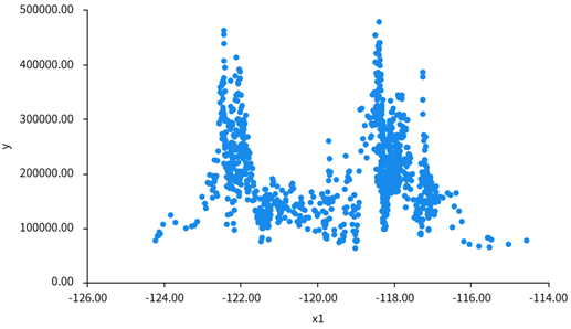
Figure 2: Scatter plot of x1 and y

Similarly, x₇ shows scattered data points with no visible patterns, suggesting that the number of households in California is not strongly predictive of housing prices in this dataset (Figure 3).

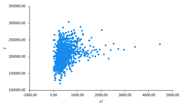
Figure 3: Scatter plot of x7 and y

3.2. Correlation analysis

To further quantify the correlation between the variables, an additional analysis is conducted using the Pearson correlation coefficients. The results are shown in Figure 4. The Pearson correlation analysis reveals several relationships between median house prices in blocks in California and the independent variables as stated. Among them, median income shows the strongest positive correlation with California house prices (0.69), suggesting a substantial association. Other variables, such as housing median age (0.11), total rooms (0.13), total bedrooms (0.05), and households (0.07), also show positive correlations with the dependent variable, though weaker in magnitude.

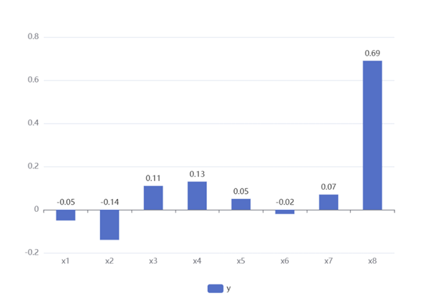
Figure 4: Relevance between independent and dependent variables

Conversely, latitude (-0.14), longitude (-0.05), and population (-0.025) demonstrate significant negative correlations with California house prices, indicating inverse relationships. Despite their statistical significance, the correlation strengths remain relatively weak, except for median income, which stands out as the most influential factor. These findings highlight the need for further analysis and perhaps transformation of these variables before incorporating them into a regression model.

3.3. Multiple Linear Regression (MLR) analysis

The results of multiple linear regression analysis are shown in Table 2:

Table 2: MLR results (n=20433) 

From Table 2, the formula of the model can be obtained:

\( y = 3585395.747 - 42730.120x1 -… + 40297.522x8 \) (2)

The value of R² is 0.637, suggesting a good fit of the model and that the independent variables explain 63.7% of the changes in California house prices. The results show that x3, x5, x7, and x8 have a significant positive impact on y, while x1, x2, x4, and x6 have a significant negative impact on y. The multicollinearity test for the model reveals that the VIF values for x4, x5 and x7 exceed 10, indicating the presence of collinearity issues, which could be resolved by applying stepwise regression or ridge regression further. In addition, P values, which explain the significance of the results, are all 0.000. This indicates that the independent variables have significant impacts on housing prices in California.

The multiple linear regression analysis was performed on a substantial sample of 20,433 observations, yielding an R² of 0.637 and indicating that approximately 63.7% of the variance in the dependent variable is explained by the predictors. The intercept was estimated at -3585395.747, which, given the measurement scales involved, requires cautious interpretation. All predictor variables (x1 through x8) exhibited statistically significant effects (p < 0.001). The standardized beta coefficients reveal that x2 (β = -0.787) and x1 (β = -0.742) exerted strong negative influences, whereas x8 (β = 0.663) had a robust positive effect on the outcome variable. Additionally, despite the high statistical significance of these coefficients, several predictors (notably x4, x5, and x7) displayed high variance inflation factors (VIFs of 12.717, 36.004, and 35.136, respectively), accompanied by very low tolerance values, signaling a potential issue of multicollinearity that may undermine the stability and interpretability of the coefficient estimates.

4. Conclusion

This study is based on the California House Price dataset, with 20433 usable data entries for analysis. Correlation analysis and multiple linear regression are performed to investigate factors influencing house prices in California. It is observed that median income has the most significant correlation with median housing price in California from the correlation analysis. Additionally, the linear regression model is obtained to estimate the housing prices, with a good fit of the R² value at 0.637.

During the MLR analysis in this study, the issue of multicollinearity has been found among total rooms, total bedrooms, and households. This implies that there is a strong correlation among these variables, which means they share a lot of information and influence each other, leading to the instability of the estimated regression coefficients, hence causing the model to be unreliable. Therefore, further analysis, for instance, ridge regression, can be conducted to enhance this model by eliminating highly correlated independent variables. This study excludes an independent variable of ocean proximity, which is included in the original dataset. Hence, for a more advanced housing price predicting model, this variable and other factors of blocks in California (transportation convenience, infrastructure, etc.) may be included.

References

[1]. Tsatsaronis, K. and Zhu, H. (2004) What drives housing price dynamics: cross-country evidence. BIS Quarterly Review, March.
[2]. Bohn, S. and Duan, J., (2025) California’s Economy, Public Institute of California. International Journal of Information Engineering & Electronic Business.
[3]. Park, B. and Bae, J.K. (2015) Using machine learning algorithms for housing price prediction: The case of Fairfax County, Virginia housing data. Expert systems with applications, 42(6), 2928-2934.
[4]. Nguyen, N. and Cripps, A. (2001) Predicting housing value: A comparison of multiple regression analysis and artificial neural networks. Journal of real estate research, 22(3), 313-336.
[5]. Truong, Q., Nguyen, M., Dang, H. and Mei, B. (2020) Housing price prediction via improved machine learning techniques. Procedia Computer Science, 174, 433-442.
[6]. Fedotova, O., Teixeira, L. and Alvelos, H. (2013) Software Effort Estimation with Multiple Linear Regression: Review and Practical Application. J. Inf. Sci. Eng., 29(5), 925-945.
[7]. Zhang, Q. (2021) Housing price prediction based on multiple linear regression. Scientific Programming, 1, 7678931.
[8]. Thamarai, M. and Malarvizhi, S.P. (2020) House Price Prediction Modeling Using Machine Learning. International Journal of Information Engineering & Electronic Business, 12(2).
[9]. Coulson, N.E. and Daniel P.M. (2008) Estimating time, age and vintage effects in housing prices. Journal of Housing Economics, 17, 138-151.
[10]. Sani, M.M. and Rahim, A. (2015) Price to income ratio approach in housing affordability. Journal of Economics, Business and Management, 3, 1190-1193.
Cite this article
Gu,Y. (2025). Predicting Housing Price Using Regression Analysis: A Study Based on California Housing Price. Theoretical and Natural Science,105,128-134.
Data availability
The datasets used and/or analyzed during the current study will be available from the authors upon reasonable request.
Disclaimer/Publisher's Note
The statements, opinions and data contained in all publications are solely those of the individual author(s) and contributor(s) and not of EWA Publishing and/or the editor(s). EWA Publishing and/or the editor(s) disclaim responsibility for any injury to people or property resulting from any ideas, methods, instructions or products referred to in the content.
About volume
Volume title: Proceedings of the 3rd International Conference on Mathematical Physics and Computational Simulation
© 2024 by the author(s). Licensee EWA Publishing, Oxford, UK. This article is an open access article distributed under the terms and
conditions of the Creative Commons Attribution (CC BY) license. Authors who
publish this series agree to the following terms:
1. Authors retain copyright and grant the series right of first publication with the work simultaneously licensed under a Creative Commons
Attribution License that allows others to share the work with an acknowledgment of the work's authorship and initial publication in this
series.
2. Authors are able to enter into separate, additional contractual arrangements for the non-exclusive distribution of the series's published
version of the work (e.g., post it to an institutional repository or publish it in a book), with an acknowledgment of its initial
publication in this series.
3. Authors are permitted and encouraged to post their work online (e.g., in institutional repositories or on their website) prior to and
during the submission process, as it can lead to productive exchanges, as well as earlier and greater citation of published work (See
Open access policy for details).