1. Introduction

In the highly developed industry environment mechanical gear transmission systems exert extremely important status. It can be seen that hundreds of different gears today work in each machine. So the simulation of gear is not to be ignored, whether from the economic side or efficiency side, using computer software to simulate the gear would save lots of time and money to achieve an ideal outcome. Despite a large number of papers and books, e.g. the computational approach with the finite element method was used to determine the static transmission error [1], elements of worm gear drive design [2], dynamic contact simulations for the helical gear pairs [3], deep study 2D and 3D modification of helicalgear pair [4], static and dynamic gear mesh study on tooth [5], Gear shaping simulation for face-gears [6], and crack on gear tooth root [7] describing in detail different gear and FEA mesh problems, two of the main challenging issues were ignored, namely mesh size, mesh method and refinement on gear, are far from being jointly solved. This paper using Ansys to analyze 3 important aspects mesh size, mesh method and refinement to help people in the future use better ways to mesh a specific gear on Ansys.

2. Theory background

2.1. FEA theory

This paper sets up the Finite Element Analysis (FEA) to calculate the gear stress. FEA is a mathematical method to simulate the real-world physics system by using several simple interaction elements (unites) to achieve a finite number of unknown elements to approximate a real system with infinite unknown elements. FEA uses simple questions to answer the complicated question and then solve it. FEA treats the solution domain as consisting of many small interconnected sub-domains called finite elements, assumes a suitable (simpler) approximate solution for each element, and then derives the overall satisfying conditions (such as structural equilibrium condition) to get the solution of the problem. And it is not the exact solution but an approximate solution. So using FEA could have a highly approximate solution to the question also suitable for different complicated structures. Figure 1 explains the logic of the FEA system [8].

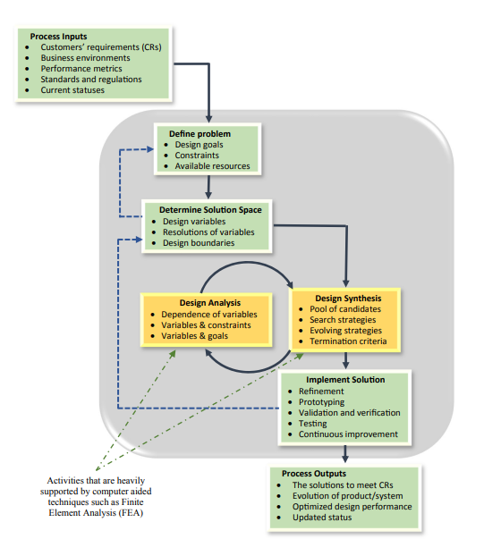
Fig. 1. FEA Logic Diagram [8]

There are 8 steps in FEA preprocessing. Step 1: Define the geometry for the problem; Step 2: Create the material model; Step 3: Choose the type of elements and mesh the model; Step 4: Define element equations; Step 5: Assemble the equations into a system equation solution; Step 6: Define the boundary conditions; Step 7: Solve postprocessing, and finally Step 8: Review the results and analyze what they mean to the real world problem [8].

Here is a mathematical equation example for spring when using FEA on it (Figure 2). By using the FEA method, this paper has clear solutions about the structure and compares to the normal real instruments to solve the problem, FEA method is more efficient by saving a bunch of time and money without doing the experiment.

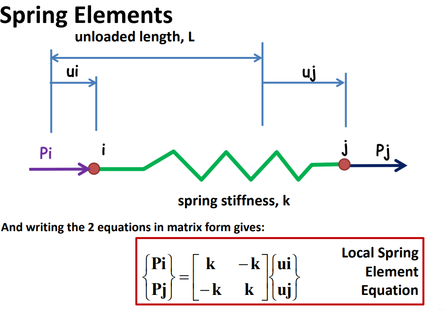
Fig. 2. The matrix equation for spring [9]

2.2. Configuration (mesh size, mesh type)

The usual way to use the FEA system is by doing it on the software. For example, ANSYS is one of the famous simulation software. ANSYS is a general-purpose software used to simulate interactions of all disciplines of physics, structural, vibration, fluid dynamics, heat transfer, and electromagnetic for engineers [8].

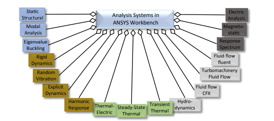
Fig. 3. Functions of ANSYS workbench

For simulation software, it depends on a lot of setups to simulate an approximate structure that is required. Lots of boundary conditions are needed to simulate in a different environment to get detailed information about the structure. For example, the division of finite element mesh such as meshing size and mesh type. When the simulated structure needs to become closer to the real world, the mesh size is needed to decrease to achieve what people want. This is because when increasing the number of elements (By decreasing the mesh size) that are meshed, more detail for the structure will be showed. Meanwhile the quantitative of calculation increase dramatically it will take lots of time to compute. To find a balance of accuracy and efficiency, simulations are conducted on a spur gear with a pitch circle diameter of 20mm with 6 different mesh sizes and different mesh types to obtain the maximum stress around the gear teeth for each submitted configuration.

2.3. Gear theory

The tooth surface contact strength includes two stress states, the tooth surface contact fatigue strength and the tooth surface contact static strength. The types of tooth surface failure can be classified into pitting, scuffing, wear, micro-pitting and fracture. Types of the strength of gears subjected to external meshing forces: fatigue strength, static strength. In this paper, the crack/fracture phenomenon under static strength failure of the tooth root is studied. The formula for calculating the stress on teeth root is shown on equation 1, In the formula \( {Y_{F}} \) is the tooth shape coefficient; \( {Y_{S}} \) is the stress correction coefficient; \( {Y_{β}} \) is the helix angle coefficient [10].

\( {σ_{F0=}}\frac{{F_{t}}}{b{m_{a}}}∗{Y_{F}}∗{Y_{S}}∗{Y_{β}} \) (1)

According to the operating state of the gear system, the calculated tooth root stress should be corrected with influence factor as is shown in the equation 2. In the formula, \( {K_{A}} \) is the application coefficient; \( {K_{V}} \) is the dynamic load coefficient, \( {K_{F β}} \) is the tooth load distribution coefficient; \( {K_{Fα}} \) is the inter-tooth load distribution coefficient \( [10] \) . With this equation can obtain the bending stress \( σF \) at gear teeth when a meshing force Ft is applied.

\( σF={σ_{F0}}∗{K_{A}}∗{K_{V}}∗{K_{Fβ}}∗{K_{Fα}} \) (2)

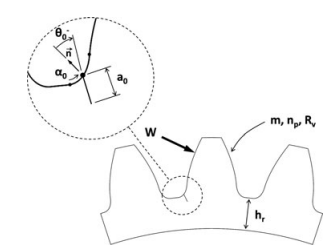
Fig. 4. Details for gear teeth root

3. Analysis and Compare of results

3.1. Discussion of Mesh size

For the research of mesh size, a dimensionless function is made for gear, D is the diameter of the gear and X is the mesh size. Function 3 is created to observe when N increases what will happens to the stress on the gear teeth root. According to the similarity principle, the same function on gear that the size of gear has not to change but change in mesh size or another variable can find out the changing pattern on it.

\( N=\frac{D}{X} \) (3)

By using different mesh sizes, D is the diameter of gear equal to 20mm and 5 different mesh sizes are chosen: 4mm, 2mm,1mm, 0.5 mm, 0.25mm and 0.1mm to obtain each of stress from different mesh sizes. At first when increasing the value of N the value of maximum stress increase too. From the trend line, the difference of increasing Maximum stress becomes less and less due to the calculation being close to the analytical solution because mesh size decrease, but also the decrease of mesh size will cost more time to calculate in Ansys.

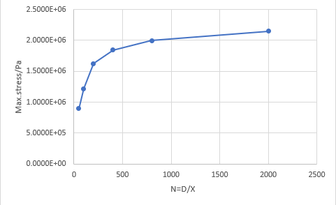
Fig 5. Max. stress vs N

As shown in Figure 5, as the dimensionless number N increases, the stress of gear increase too; and the change of stress decreases. The increment of maximum stress change by 36% from N=50 to N=100, by 33.3% from N=100 to N=200, by 13% from N=200 to N=400, by 8.26% from N=400 to N=800, by 7.62% from N=800 to N=2000. When the percentage of change of maximum stress is smaller than 10% then the N is in convergent and that correspond to N>800.

3.2. Mesh Method

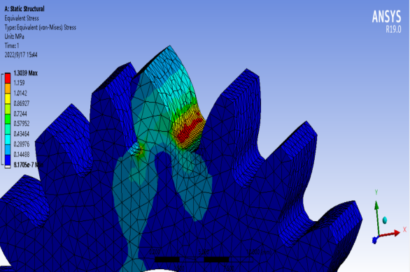
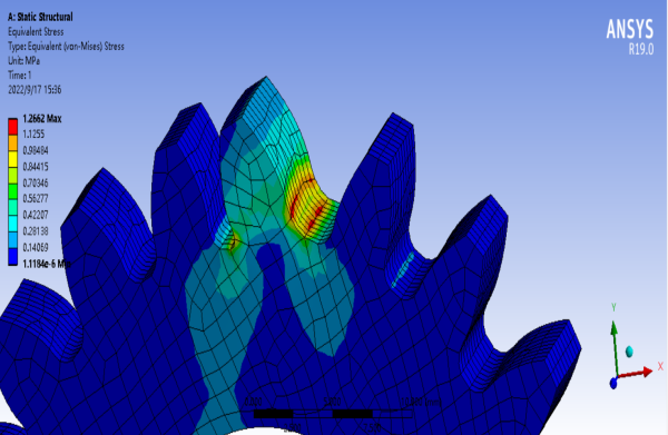
Fig. 6. Mesh type: Tetrahedrons Fig. 7. Mesh type: Hex linear

These two figures above show the difference between the mesh type in tetrahedrons and Hex linear. The most distinct observation between the tetrahedron method and the hex linear method is the stress distribution becomes more and more discrete at the gear teeth root area. This is because the tetrahedral mesh method can fit better in complex geometry than hex linear by the interpolation algorithm of the Ansys. A 3D mesh with n vertices such as in tetrahedron has 4 nodes and in hexagon has 8nodes. Point 2, 3, 4, 5 in tetrahedral (Figure 7) and point 5, 6, 7, 8, 9 (Figure 8) form a face respectively. They are the outer faces of the gear mesh and from the observation, the stress on point 9 (hex linear) is smaller than point 5 (tetrahedrons) leading to the difference in stress contour. This is because the FEA method is used to calculate the stress on linear, endpoint and quadratic but cannot calculate the stress of a point at the middle of the curve face. So, it is necessary to use interpolation to find out the stress between the nodes and nodes.

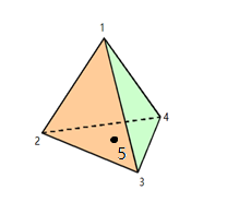
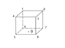
Fig. 8. Tetrahedral Fig. 9. Hexagon

A function for interpolation is show below:

\( Y=f(x1,x2,x3,……xn) \) (4)

The value of \( x1, \) \( x2 \) and \( x3 \) are the vertices values for the structure. In Ansys, the specific function for interpolation is not showing up but it must obey a rule that \( Y \) >Min ( \( x \) n) and Y<Max ( \( x \) n). For a certain f(x), when there are smaller \( x \) n, the final \( Y \) is relatively small; when there are larger \( x \) n, the final \( Y \) is relatively larger. Supposing Ansys is using average interpolation \( Y=mean(x1,x2,x3,……xn) \) and algebra for each vertex. So, the formula for tetrahedral will be formula (5):

\( {Y_{4}}=\frac{x1+x2+x3+x4}{4}, x1=x2=x3=m,x4=n，m \gt n \) (5)

The formula for hexagon will be formula (6):

\( {Y_{6}}=\frac{x1+x2+x3+x4+x5+x6+x7+x8}{8},x1=x2=x3=x4=m,x5=x6=x7=x8 =n,m \gt n \) (6)

From formulas 5 and 6, the interpolation value of stress for point 5 (tetrahedral) is bigger than point 9 (hex linear) and therefore tetrahedral mesh method is better in complex geometry compared to the hex linear at certain mesh size while mesh is refined this difference can be diminished.

3.3. Refinement of mesh

By adding refinement at the gear teeth root, more details from Ansys is observed from different mesh size. According to four different refinement levels in 0.5mm global mesh size and 0.25mm global mesh size, the most difference between the 0.5mm mesh size and the 0.25mm mesh size is the stress change between refinement level 1 and refinement level 2, and makes the trend line is not that linear as mesh size 0.25mm, this is because the huge difference stress data from the no refinement, refinement level 1 and refinement level 2 as the mesh size is too big, so the divergence appears in data from the calculation.

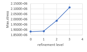
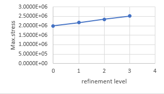
Fig. 10. Mesh size 0.5mm Fig. 11. Mesh size 0.25mm

4. Conclusion

Overall, this document analyze 3 field differences in gear simulation by using Ansys. Mesh size is always a big problem because the mesh goes smaller the time and the cost gets longer so from the experiment N=800 would be a suitable mesh size for calculating the stress. For the mesh method in this kind of complex structure especially at the gear teeth root the tetrahedral mesh method would be a better choice than other normal mesh methods because the interpolation of the tetrahedral method can better simulate the real world simulation. Refinement is a good way to observe more detail in certain areas and it is better to use a small mesh size (<0.25mm) to get approximate data from Ansys. This paper analyzes 3 different aspects of the Ansys mesh system to help people get a better choice on how to mesh a gear in a different environment in the future.

References

[1]. Alexander Czakó, Kamil Řehák, Aleš Prokop, Vinayak Ranjan, Determination of static transmission error of helical gears using finite element analysis, 2020.
[2]. Jelaska D. Gears and Gear Drives. Wiley, Chichester, 2 012, pp.421-422.
[3]. Yongjun Wu, Jianjun Wang and Qinkai Han, Static/dynamic contact FEA and experimental study for tooth profile modification of helical gears [J] Journal of Mechanical Science and Technology, 2012, 26 (5) 1409-1417.
[4]. P. Wagaj and A. Kahraman, Influence of the tooth profile modification on helical gear durability, Journal of Mechanical Design, 2002: 123.
[5]. Hui Wang, Yiming Rong, Gong H., Zhou, J. Spur gears static and dynamic meshing simulation and tooth stress calculationJammal, EDP Sicences, 2015.
[6]. H. Andreas Zschippang, Sascha Weikert, Konrad Wegener, Face-gear drive: Simulation of shaping as manufacturing process of face-gears, ELSEVIER, 2022.
[7]. Pehan, B. Zafošnik and J. Kramberger, CRACK PROPAGATION IN GEAR TOOTH ROOT S. University of Maribor Slovenia, Maribor, Smetanova 17, 2000.
[8]. Finite element analysis applications: a systematic and practical approach, Zhuming Bi, Chapter 1, ScienceDirect, 2019, pp.2-7.
[9]. C. Charlie, L. Wang, MS2_FEA_Lec03_Spring&BarElements.pdf, 2021.
[10]. ISO, ISO 6336-3:2019 Calculation of load capacity of spur and helical gears-Part 3: Calculation of tooth bending strength, November 2019, https://www.iso.org/standard/63822.html.
Cite this article
Lin,K. (2023). Static gear research of mesh simulation based on Ansys. Theoretical and Natural Science,5,575-581.
Data availability
The datasets used and/or analyzed during the current study will be available from the authors upon reasonable request.
Disclaimer/Publisher's Note
The statements, opinions and data contained in all publications are solely those of the individual author(s) and contributor(s) and not of EWA Publishing and/or the editor(s). EWA Publishing and/or the editor(s) disclaim responsibility for any injury to people or property resulting from any ideas, methods, instructions or products referred to in the content.
About volume
Volume title: Proceedings of the 2nd International Conference on Computing Innovation and Applied Physics (CONF-CIAP 2023)
© 2024 by the author(s). Licensee EWA Publishing, Oxford, UK. This article is an open access article distributed under the terms and
conditions of the Creative Commons Attribution (CC BY) license. Authors who
publish this series agree to the following terms:
1. Authors retain copyright and grant the series right of first publication with the work simultaneously licensed under a Creative Commons
Attribution License that allows others to share the work with an acknowledgment of the work's authorship and initial publication in this
series.
2. Authors are able to enter into separate, additional contractual arrangements for the non-exclusive distribution of the series's published
version of the work (e.g., post it to an institutional repository or publish it in a book), with an acknowledgment of its initial
publication in this series.
3. Authors are permitted and encouraged to post their work online (e.g., in institutional repositories or on their website) prior to and
during the submission process, as it can lead to productive exchanges, as well as earlier and greater citation of published work (See
Open access policy for details).