Analysis on Gliese 486 b

Zhihui Zhou^1*, Jiatong Li², Yutong Zhong³, Zhongqian Hou⁴, Ruixi Yao⁵

¹College of Science, Northeastern University, Boston, 02115, the United States pf America

²International Department, ShenZhen Middle School, Shenzhen, 518010, China

³Beijing National Day School, Beijing, 10039, China

⁴Qingdao No.9 High School,266000, China

⁵University of Queensland, Birsbane, 4067, Australia

* Corresponding author. Email: melissazhou579@gmail.com.

Abstract. Gliese 486 b, also known as GJ 486 b, is an exoplanet orbiting around a red dwarf near our solar system. The celestial body is fair target for TESS to observe and related data of it have been collected by TESS. This paper firstly focuses on methods used to obtain planetary parameters and the theoretical base behind them. Then, it turns to some further calculation with our best-fit data, and analogy to the methods that previous researches used. Finally, the paper introduces analysis on the changing period and the relevant potential causes. The paper concludes with some discussion on directions of future investigations.

Keywords：Gliese 486 b, transit, coding, tidal effect, period change.

1. Introduction

The object of observation in this work is GJ 486 b, an exoplanet that rotates around GJ 486, a red dwarf star near our solar system, and the host star is only 8 pc from the sun. GJ 486 was discovered by Wolf in 1919 with basic photographic plates collected with the Bruce double astrograph on Königstuhl, Heidelberg. But the planet was not discovered until 2021 by Trifonov et al [1]. The planet is a terrestrial planet, more precisely, an earth-like planet whose mass is of 2.81 Earth masses and has a radius of 1.31 Earth radius, with uncertainty of 5% [2]. Its overall density is close to that of Earth and Venus, making it an example of Super Earth. Compared with earth, it has a shorter orbital period and correspondingly higher equilibrium temperature, orbiting around a brighter, cooler and less active stellar host [2].

The reason of choosing GJ 486 b as target is because that its condition is relatively great for observation and data analysis, compared with other known exoplanets. Several factors make it easy to detect: The host star system, GJ 486 is not only a detectable target of TESS, but also the third-closest transiting exoplanet system known. The red dwarf is small and of low mass, which makes the exoplanet around it easy to detect, as the up-and-down trends in its radial velocity and light curves are easy to detect and measured. Affected by the factors above, GJ 486 b become the closest transiting planet around a red dwarf with a measured mass. In addition, though GJ 486 is not hot enough to be a lava world, caused by the coolness of its host star, its temperature, which is of roughly 700K, makes it suitable for emission spectroscopy and phase curve studies in search of its atmosphere [2].

2. Coding Methods

2.1 Model

Lightkurve is the resource library where the data of GJ 486 b are obtained, among which data 0 and data 5 are analyzed and compared since they are both observed by the author SPOC, and their exposure time are 120, which is relatively accord with our expectation. In the following paper, data 5 is used as an example to illustrate the coding methods, and data 0 is processed the same.

The “occultquad” function from Mandel & Agol is used as the model of light curve[3]. It contains 4 parameters: t0, k, a, period. Being defined as transit_lightcurve(t, *parameters) where u equals to 0.16 and b equals to 0.45, the six parameters are expressed in the following relations:

phi = 2.*np.pi*(t-t0)/period is the phase of the orbit.

x = a*np.sin(phi) is the x-coordinate with reference to Fig. 2 of Winn (2010).

y = b*np.cos(phi) is the y-coordinate with reference to Fig. 2 of Winn (2010).

s = np.sqrt(x*x + y*y) is the distance between planet and star on the sky.

flux_calc, flux_no_limb_darkening = occultquad (s, 0.16, 0.45, k) is used to calculate the loss of light.

flux_calc[y<0.0] = 1.0.

2.2 Limb Darkening Coefficients

Parameters u and b are typically set into two constants instead of variables. These two constants are the limb-darkening coefficients (LDC) for GJ 486 b’s host star GJ 486, which is a star with radius of 0.33 Rsun and temperature of 3297K. According to Claret A., in 2018, a star with temperature of 3297K, that is, approximately 3300k, and log g value of \( 4.81±0.12 \) (from table 2 of 2022 GJ486), has LDCs of 0.45 and 0.16, for parameters b and u respectively, calculated by equation 2 [4-6]. There are two reasons for setting these two parameters into constants: 1. Having six variables at the same time to require Python to fit the parameters may cause some unnecessary error to the curve fit of transit light curve; 2. GJ 486 is not a sun-like star, so the initial guess of the parameter u cannot simply be set into 0.6 just as other exoplanet of a sun-like star.

2.3 Folding

After downloading the desired data set, a process to eliminate points defined as Not a Number (NAN) is conducted in case of the computer reporting errors in the following fitting. To this end, a Boolean array is created in which ok is defined as np.isfinite(f) and t is set to be t[ok], f to be f[ok]. The Boolean array is true whenever the flux is finite; it is false whenever the flux is not finite. When the array is false, the time t is taken and replaced by the subset of times that are finite.

Folding the data to check whether the planet has clear and definite transits is also necessary. Values of conjunction time and period are, from Trifonov et al. 2021, tc =2458931.15935 – 2459600, and period=1.467119. Then, t_folded is defined as the folded time[1].

Time t is used to minus tc_est and subtract integer number of orbits that have elapsed since tc_est multiplied by p_est. This folded time that subtracts a certain integer number of orbital periods from the estimated transit time is now a variable that runs between 0 and the orbital period. The code of t_folded is defined as follow:

\( {t_{folded}}= (t-t{c_{est}})- {p_{est}}*np.floor(\frac{t-t{c_{est}}}{{p_{est}}})…(1) \)

After subtracting the data with a whole period so that the data centers at 0.0, the transit is defined as the range in which the absolute value of t-folded is less than 0.04. All of the data points that span the transit of the planet are now successfully identified, which also makes it easier to distinguish the data points outside transit. From Figure 1, a whole transit is shown clearly (red dots), indicating that this planet can be treated as a normal transit planet to study and analyze.

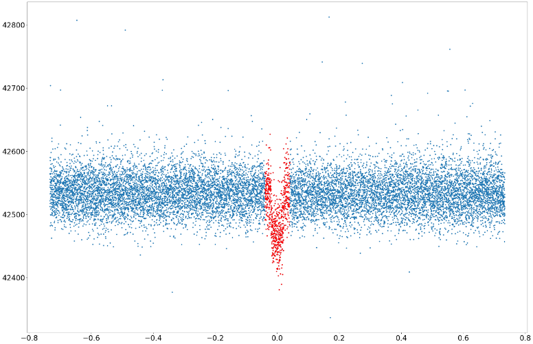
Figure 1. Data points of data 0 after folding.

2.4 box least square (BLS) method

The BLS method recognizes the transit light curve as a periodic upside-down model with four parameters: period, duration, depth, and a reference time. In this regard, the reference time can be considered as the mid-transit time of the first transit in the observational baseline. Figure 2 is a diagram illustrating the 4 parameters.

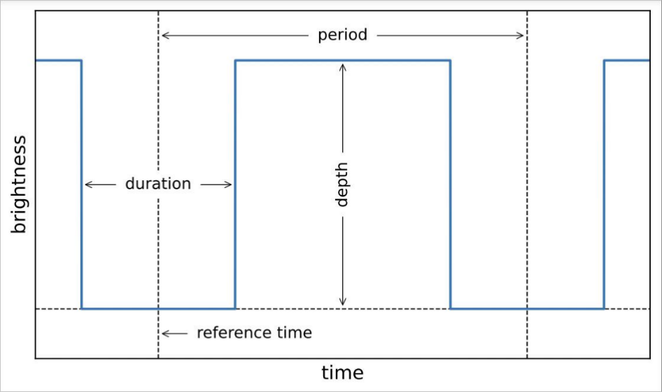
Figure 2. Simplified illustration of how BLS works [7].

The BLS periodogram is a statistical tool used to detect the period and conjunction time of the transiting exoplanets in light curves. This method displays a Jupyter Notebook Widget which enables the BLS algorithm to be used interactively. Periodogram is a method to estimate the signal power spectral density. To get the estimated value, the signal sequence needs to complete a discrete Fourier transform, and the square of its amplitude-frequency property will be divided by the length of the sequence (N). Matplotlib is a tool used here to help plotting the result. Figure 3 and Figure 4 show the BLS diagrams and parameters for data 0 and data 5.

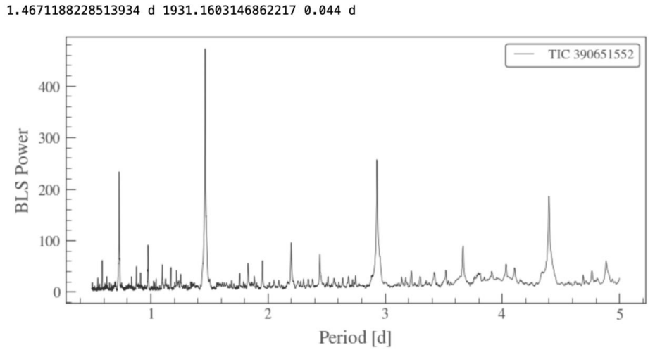
Figure 3. BLS result for data 0.

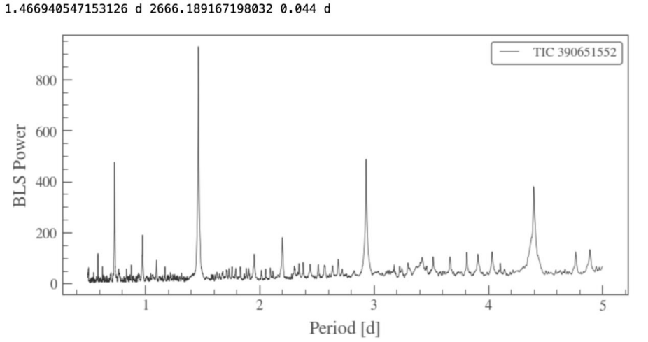
Figure 4. BLS result for data 5.

2.5 calculations of the uncertainty

To do a curve fit, which requires the uncertainty to fit the parameters, the noise level, or the uncertainty, of the data from a segment outside any transit needs to be calculated. In addition, the data also need to be normalized by dividing them by their median so that all the data on the vertical axis are normalized to the axis centered on one. To achieve this, a segment outside any transit from t=85.3 to 86.6 (after shifting the graph of 2459600) is defined and the median of the data in the segment is found. Being divided by their median in the segment, the values of flux in the segment is normalized, with the range from approximately 0.997 to 1.003 according to Figure 5. The uncertainty is then the standard deviation of the selected and processed data. However, the required uncertainty should not simply be a value, but an array of values. Thus, t is multiplied by 0.0 and added the uncertainty to each value to get an array with the same length as t and the same value as uncertainty.

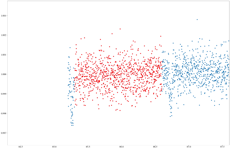
Figure 5. Selected points between two transits (data 0).

2.6 Parameter fitting

Parameters are ready to be fitted with our initial guesses after calculating the uncertainty. For data 5, the initial guesses of parameters are: tc =2668.55, k= \( \sqrt[]{0.0022} \) , a=10.0, and period=1.466940547, in which tc, k and a are adjusted many times according fitted results, whereas period takes the value calculated by BLS method above. The final result of the fitting generated by curve fit method is shown in Figure 6, and the parameters are: tc= 2.66864033e+03+-3.12569551e-03, k=3.71934016e-02+-4.75723657e-04, a= 1.02916005e+01+-1.06883937e-01, and period=1.46699658+-1.76399154e-06.

Figure 6. Curvefit of data 5 after parameter fitting.

The final results of parameter fitting for data 0 are: tc=1.93116784e+03+-5.05268676e-03, k=3.67322058e-02+-5.03076826e-04, a=1.02615938e+01+-1.16907299e-01, and period=1.46718853+-3.92446398e-06.

2.7 Chi-square value

Finally, the values of chi-square and the max expected chi-square of each fitting is calculated to check the accuracy of the fitting. If the value of chi-square is at the same order of magnitude as the maximum expected value, the fitting is fairly good; if not, the fitting method may need to be improved. In the case of data 5, chi-square value for data 5 is 11673.725748376055, and the max expected value is 10965.091808065576, which is at the same order of magnitude chi-square value, indicating that our fitting is acceptable. It is the same for data 0, which has a chi-square value of 17594.678193835884 and a max expected value of 13325.252889034371.

2.8 Flattening attempts made to fit the data better

Another method Flattening is also tried to fit the data. Flattening is a method to get rid of the influence of background noise. Window length is a positive odd integer that refers to the length of the filter window. Periodical blank can be observed in the residue graph of the data after flattening when window length is set to be 201, so attempts were made by trying several other positive odd integral numbers and found out that the diagram with window length of 1001 is better, as the data is distributed more randomly and independently. Figure 7 and Figure 8 are the residue graph when window length equals to 201 and 1001.

Figure 7. Window length=201(result 0).

Figure 8. Window length=1001(result 0).

Polyorder stands for the highest order of the polynomial used to fit the samples. The value of polyorder must be smaller than the window length. Linear fitting is not suitable for the data itself, since bac ground noise can hardly have such regular fitting like this. Using a polyorder larger than 2 could also receive a great outcome. However, this may decrease the signal too much that some extra details of the dataset will be cut as well. As shown in Figure 9 and Figure 10 respectively, the polyorder is set to be two.

Figure 9. Data plot after flattening (data 0).

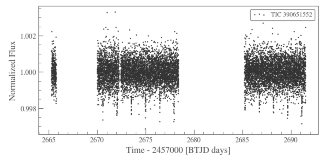
Figure 10. Data plot after flattening (data 5).

The residue graph is used to check if the residuals are independent and random. It is clear that flatten method adjust the data slightly to make its residuals more independent and random. Figure 11 and Figure 12 are the plot of the residuals.

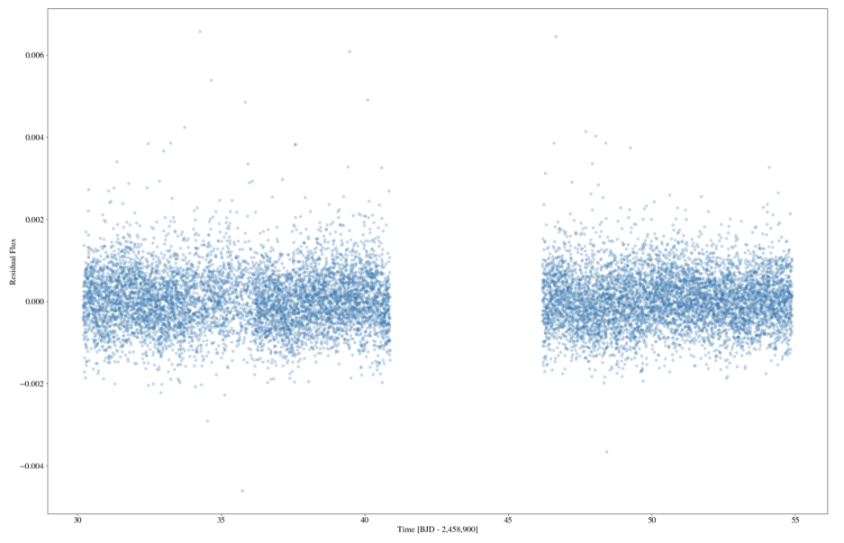
Figure 11. Residue graph of data 0 BEFORE flattening.

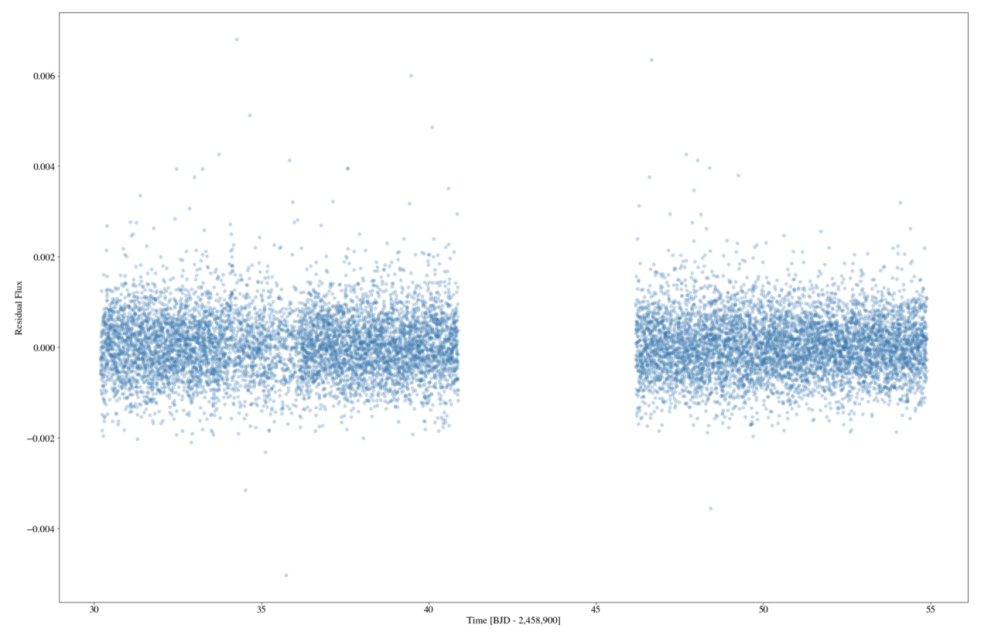
Figure 12. Residue graph of data 0 AFTER flattening.

By comparison, the light curve after flattening is more independent and normal. As the limb darkening parameter u and transit impact parameter b is set to be constants (0.16 and 0.45). The final curve fit result has 4 parameters, corresponding to the midpoint of transit with time shift, the value of the radius of the planet over the radius of the star, which is “k”, the ratio of the orbital radius and the stellar radius, which is “a” and the period of the transit.

Initial curve fit of result 0

Best fitting parameter values:

[1.93116784e+03 3.67322058e-02 1.02615938e+01 1.46718853e+00]

Uncertainties:

[5.05268676e-03 5.03076826e-04 1.16907299e-01 3.92446398e-06]

Curve fit of result 0 after flattening

Best fitting parameter values:

[1.93112121e+03 3.56481165e-02 1.03428279e+01 1.46715230e+00]

Uncertainties:

[5.56064103e-03 5.16643797e-04 1.21865384e-01 4.30253788e-06]

Initial curve fit of result 5

Best fitting parameter values:

[2.66864033e+03 3.71934016e-02 1.02916005e+01 1.46699658e+00]

Uncertainties:

[3.12569551e-03 4.75723657e-04 1.06883937e-01 1.76399154e-06]

Curve fit of result 5 after flattening

Best fitting parameter values:

[2.66861258e+03 3.62998601e-02 1.03562610e+01 1.46698086e+00]

Uncertainties:

[3.50887667e-03 4.83351093e-04 1.11579579e-01 1.99242375e-06]

Being Compared to the result of uncertainty of before flattening (the initial data), the uncertainty after flattening is relatively larger than it but the value derived is really closed. The initial data is more accurate. The most obvious difference between result 0 and result 5 is the conjunction time. The reason of the large difference is that the telescope derived the two results with a period of time in between.

3. Further Calculation

The computational component is essential to understand the internal composition of the planet and to calculate the orbital period of the planet by the time between transits with measurements of the stellar size and the depth of brightness decrease [8]. The orbital period of an exoplanet depends on whether the planet transits its primary star at the edge or at the center, where it may be necessary to "flatten" the light-change curve to correct for the intrinsic variability of the star. For planets with greater radii, the brightness of these stars will be significantly dimmer, and the greater radii of transiting gas giants will dim the brightness of these stars even more. Such information is crucial for the understanding of the internal composition of these planets. This work assumes that the detection probability is a function of the observed S/N, which is calculates in the case of TESS [9].

Time between transits can be applied to compute the planetary orbital period, so once the orbital period is determined the average separation between a planet and its star can be calculated from Kepler's third law of planetary motion. The size or radius of the planet is calculated from the size of the star derived by measuring the depth of the decrease in brightness. The radii of expanding hot Jupiters due to the radiation of the host star are significantly larger than the mean radius of Jupiter, and they can be identified from continuous, high-quality photometric profiles given the measurement of the radius of the host star. Besides, these stars become much fainter for expanding radii and expanding transit gas giants. To the extent that the valuation of planetary radii comes directly from measurements of planet-to-star radius ratios during transit events, the uncertainty in the measurements is greatly reduced by unknown systematic errors, varying methods of transit light curve analysis, or incomplete data sets.

A great deal of data is necessary to obtain an understanding of the internal composition of these planets, whereas the study by Brady and Bean offers a precise estimate of the radii of the planets, which combined with highly accurate RV observations can yield predictions of the masses and mean densities of the planets [10]. The accuracy of radius estimates and the separation of planets from their hosts gives info on the equilibrium temperature and gravitational potential of the planets. Assuming the scenario exists, these simulations yield estimates of exoplanet atmosphere sizes that are valuable in transmission spectroscopy. (Transmission spectra, as the radius ratio of planets to stars, were examined over the entire range of observed wavelengths to accurately characterize this feature). The orbital configuration of the system strongly contributes to the computational radius of exoplanets. The accuracy of the transit depth determination depends strongly on whether the planet is transiting its host star at the edge (b = 1) or at the center (b = 0). At this point, the expected signal-to-noise ratio (S/N) could be identified for each planetoid with the predicted TESS transit depth, total noise, and orbital period.

Assuming that the probability of detection is as a function of the SNR observed, the time and depth of each transit, the number of transits, and the contamination level of the surrounding stars are all accounted for in the signal strength calculation. Detection is possible if the signal exceeds 7.3 (.7.3 SNR) times the TESS photometric noise level and a minimum of two transits are observed.

It is found that the most likely period and conjunction times and their uncertainties by extracting the times and fluxes from the TESS data. Then calculations are made to compute several basic parameters: t0 = midpoint of the transit, k = (planetary radius)/(stellar radius), a = (orbital radius)/(stellar radius), b = transit impact parameter, and u = limb dimming parameter (0 for uniform intensity, 0.6 for solar-like) period. Furthermore, these parameters are used to infer other different properties: the phase x-coordinate of the orbit, the y-coordinate and the distance between the planet and the star in the sky. In particular, flux_no_limb_darkening and flux_calc assist in the calculation of the loss of light, where flux_calc reveals that the inclination occurs only if the planet is ahead of the star.

The results derived from Tess is plot out in order to predicted their time-shift values with preliminary speculations on the parameters, fitted the curves to obtain the values of (t0, k, a, period)

1.93130870e+03, 3.63213775e-02, 1.02469668e+01, 1.46729865e+00 with uncertainties of

[1.04616654e-02 5.92718993e-04 1.21988371e-01 8.17086728e-06].

Mass :2.82 Earths

Planet radius =1.305 x Earth

Eccentricity = 0.05

Orbital radius= 0.01734 AU

Orbital Period=1.5 days

The existence of the planet is convinced because of TESS data, enhance the accuracy of the measured orbital period, refine the measurement of the planet's radius or resulting overall density, with confirmation of any variations in the orbital period potentially induced by tidal or other forces. Simultaneously, coding gives a light curve model, and then tested our algorithm in the previously examined TESS region.

4. Analogy

4.1 A previous method to calculate parameters of GJ 486 b

The following part is written based on the paper “A detailed analysis of the Gl 486 planetary system.”[5]

4.1.1. Parameters and definitions

Orbital period (P)

Relative planet-to-star size e (p ≡ Rb/R⋆)

Time of transit center of the planet (t0, b),

Inclination of the planetary orbital plane (ib)

Star-planet separation-to-radius ratio (ab/R⋆)

4.1.2. Method

Table 1. Log-evidence and number of parameters of RV+transit juliet

modelsa [5]

Notes. (a) Models - Ipl: one planet. e: non-circular orbit. GP: Gaussian process (Prot,GP).

In Table 1, ln Z is corresponding values of Bayesian log-evidence, and Npar is number of parameters. The third model 1pl+GP and fourth model 1pl+e+GP both have relatively high values of ln Z, but since |ΔlnΖ| of third model and fourth model only vary about .5, the third model is chosen to fit GJ 486 b, for its lower value of Npar than the fourth model. For more details of ln Z value, please refer to “A detailed analysis of the Gl 486 planetary system”[5]

For the third model, the GP value centered on 49.9 d and width 10.0 d calculated by advanced computer from the photometric analysis will be used.

Then, the equation, a quasi-periodic kernel introduced by Foreman-Mackey et al. of the form,

is formulated below:

\( {k_{i,j}}(τ)=\frac{{B_{GP}}}{2+{C_{GP}}}{e^{\frac{-τ}{{L_{GP}}}[1+{C_{GP}}+cos{\frac{2πτ}{{P_{rot}}}}]}}…(2) \)

where \( τ=|{t_{i}}-{t_{j}}| \) is the time lag, \( {B_{GP}} \) and \( {C_{GP}} \) define the amplitude of the GP, \( {L_{GP}} \) is a timescale of the amplitude modulation of the GP, and Prot is the period of the quasi-periodic modulations. In order to simplify the GP equation, the parameter CGP is fixed to 0 and, therefore:

\( {k_{i,j}}(τ)=\frac{{B_{GP}}}{2}{e^{\frac{-τ}{{L_{GP}}}[1+cos{\frac{2πτ}{{P_{rot, GP}}}}]}}…(3) \)

After calculating it, five basic parameters are obtained, then many derived parameters. All parameters obtained are in Table 2.

Table 2. parameters gained by this method [5].

However, this method is extremely complex, and a super advanced computer is needed for calculation for more than a couple of weeks. Therefore, this work conducts simpler techniques introduced in previous parts to fit the parameters.

4.2 detection tools

Another reason why the other researchers can give a more precise result is because they use a better telescope called CHEOPS.

4.2.1 CHEOPS

CHEOPS (CHaracterising ExOPlanets Satellite) was launched on 18 December 2019, it is the first Small-class mission in ESA's comics vision science programme, with a purpose of determining the size of known extrasolar planets, which will allow the estimation of other characteristics of those planets.

4.2.2 TESS

This work uses data observed by TESS, also called Transiting Exoplanet Survey Satellite. It is a space telescope for NASA’s explorer program to search exoplanets with transit method. It was launched on 18 April 2018. A big difference between these two telescopes is the diameters of their main telescopes. The diameter of CHEOPS’s main telescope is 32 centimeters, but TESS only has a diameter of 10.5 centimeters.

That is not surprising because CHEOPS is designed in 2019 to correct those errors caused by low-precision like TESS telescope which is designed and launched in 2018, whose mission is only to find some obvious exoplanets with short periods and big masses from a very large space in the universe. For example, one kind of planet is called hot Jupiter, which can be found in reports of TESS telescope mission. But that doesn’t mean there are more hot Jupiters in the universe. According to the plan of the TESS mission, the TESS telescope observed a direction for a very short period, compared to the orbits of most planets or exoplanets. They only detect exoplanets that are easy to find, indicating the planets TESS finds usually have big bodies and short periods. Thus, planets hot Jupiters are most likely to be found. Overall, TESS telescope plays a big role in finding new planets; but on the other hand, the precisions of those data about the planets found must be sacrificed for the efficiency. So that is why the CHEOPS is designed in Europe for a totally different purpose-precision. If some parameters about a particular planet is desired to be calculated, CHEOPS can actually help more.

5. Analysis to Period Change of GJ 486 b

5.1 Potential causes of periods’ changes

In theoretical circumstances, planets and their host stars are eternally surrounding their common center of mass in elliptical orbits with constant periods. However, this is only valid if this work is neglecting the gravitational interaction between stellar systems and occurrences of accidental guests like asteroids and comets, while considering all the planets and stars as mass points labeled with numbers. In fact, things in real life are all complex and almost nothing is able to stay constant forever. There are many factors that can, slightly or significantly, changes the orbital period of stellar systems. According to the degree that they affect the orbital periods, the factors can be approximately categorized into two kinds—significant factors and slight factors.

5.1.1 Significant factors:

These kinds of factors can obviously affect the orbital periods of stellar systems significantly, which can be observed by viewing the stellar host’s light curve or the graph of radial velocity. The classical examples are planets coexisting in the planetary system, shifting each other’s position in orbits with gravitational force. These kinds of factors, such as the former one, occur periodically. If one subject’s transit light curve and radial velocity curve shows peculiarly dramatic fluctuation, you tend to find it periodical if you keep on checking it.

5.1.2 Slight factors

These factors are able to affect stellar systems constantly and slightly, and the effect they cause can’t be obvious unless a fairly long period is experienced. One example is the tidal effect. There is also interference caused by the gravitational force applied among multiple stellar systems near each other, but as the distance between them is too large so the interference is weak enough to be neglected.

5.2 Data analysis

All the data has been gained by using the best-fit model, including tc, the conjunction time of the transit which is used to fit the function, a, the ratio of the stellar radius to the orbital semi-major axis, k, the ratio of the stellar radius to the planetary axis, and per, the orbital period of Gliese 486 b surrounding its host star. As there’s only one regularly periodic declination on the light curve of the target and no obvious change can be seen, this work expels all the significant factors, which means that no large asteroids or comets came across Gliese 486 through the observational period, and the stellar system involves only one planet—Gliese 486 b. Now those slight factors can be studied, which, in this case, is tidal effect, the inherent factor of every single stellar system. The last part has shown that the dp/dt, rate of period changing caused by tidal effect, can be calculated. As a result, the purpose of this work is to find the real rate of period changing of Gliese 486 b with all the data available and determine if it lies in the expected range. If not, the reason will have to be found out.

5.2.1 dp/dt

2020, the other in 2022—there are two sets of result. The two light curves are the only available data of Gliese 486 b, as it’s a new-discovered target. In order to gain a better result of dp/dt, three additional sets of data—two from Trifonov et al 2021, one from a relevant paper written in 2022 are obtained[1,5].

After collecting all the data, a data table is created, with a Period versus Conjunction time graph that shows all the data points. As the target is a new-recorded exoplanet, only TESS has recorded its data. As the only available data of Gliese 486 b are the two light curves recorded by TESS, the former results in NASA Exoplanet Archive and the paper must be based on the same initial data. Owing to that, it’s not rational to consider the former results as different available data which can be used to calculate the ratio of period change. However, it can still be used to compare with the result. As Figure 13, the data is in the ranges of the two nearby data’s’ uncertainties, which reinforces the reliability of the result. The reason why its range of uncertainty is much narrower than that of the two nearby results (which is collected on Archive) is that b, the transit impact, which represents the degree that the transit deviates the stellar host’s central axis and the limb darkening factor are fixed while former groups of researchers used more sophisticated model with larger ranges of uncertainties. The rate of period change determined with the calculated results is 「-31989175e-07.」The uncertainty range of dp/dt is unable to obtain because there are only two data points available, which is too scarce to determine the uncertainty range. Figure 14 shows the graph of the data set linearly.

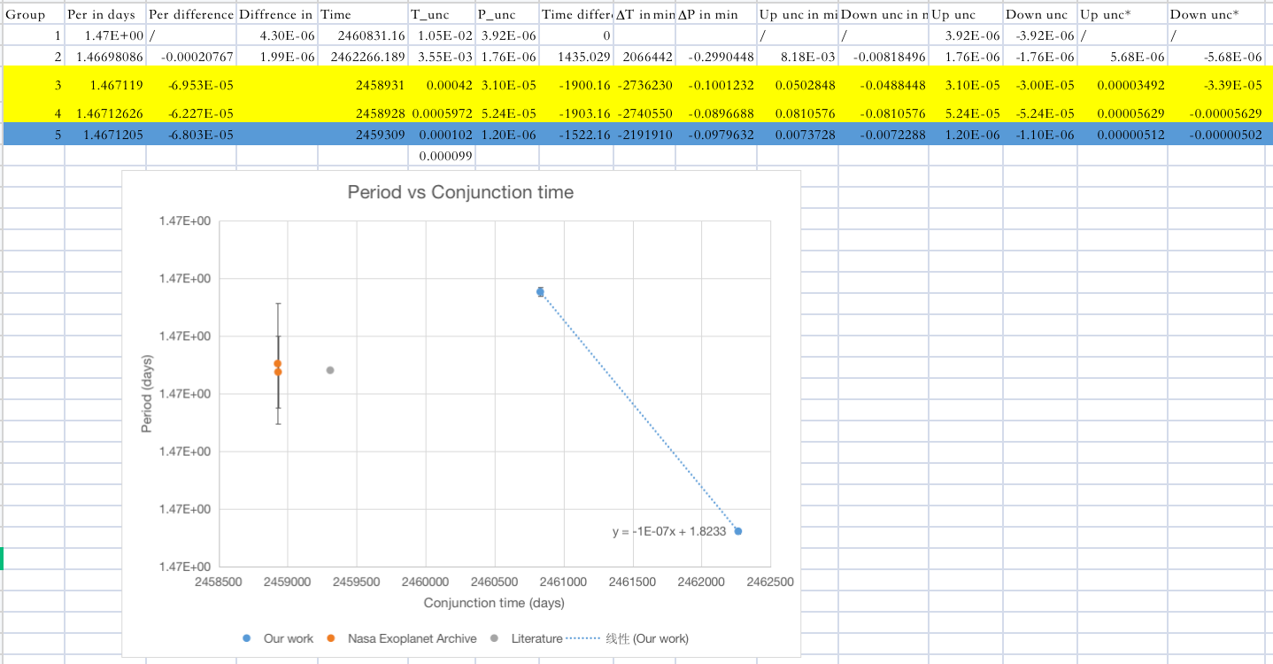
Figure 13. The data table.

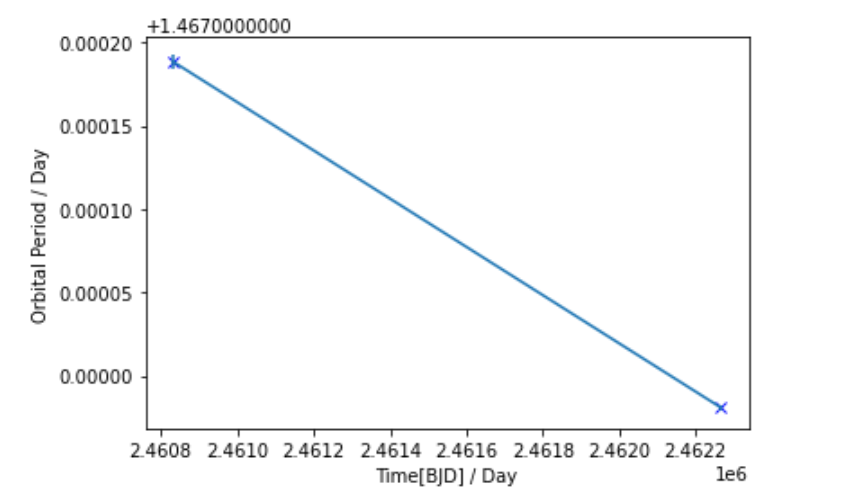
Figure 14. The data points.

The reason why a ∆Period versus ∆Conjunction time is drawn is that the numerical result would be too large and allocated broadly in this case, making the numerical size of each unit hard to decide. A logarithmic graph can definitely solve this problem, but it’s not able to reveal the linear relationship between the data directly. As a result, the original results of periods and conjunction times are set in units of days.

5.2.2 Theoretical expectation and potential factors

The Impact that tidal effect acts on the orbital period, according to former researches, has a predictable range. From the paper written by a group of astrophysicists led by Kishore C. Patra and Joshua N. Winn in 2020, the group gains the relevant formula which is abundant for prediction of dp/dt, which represents the rate of change of the orbital period of a stellar system which is only under the impact of tidal effect [11]. The formula is shown below:

\( \frac{dp}{dt}=-\frac{27π}{2{Q_{*}} \prime }\frac{{M_{p}}}{{M_{*}}}{(\frac{{R_{*}}}{a})^{5}}…(4) \)

where \( {Q_{*}} \prime \) represents the stellar tidal quality factor, \( {M_{p}}{,M_{*,}}{R_{* }}and a \) represent the planetary mass, stellar mass, stellar radius and orbital semi-major axis of the stellar system separately. \( \frac{{R_{*}}}{a} \) can be expressed in \( {α^{-1}} \) , where a is one of the results contained by the best-fit model, which is explained early in this part. The magnitudes and the resources of the derived parameters are shown in Table 3. For stellar system Gliese 486, all of the required data are already solved, except for \( {Q_{*}} \prime \) , which cannot be determined at present, meanwhile having a range of magnitude at [1,1000000].

Table 3. relevant data [1].

After Calculation, the final prediction of dp/dt in Gliese 486 system is:

\( dp/dt ∈ [(-9.7±0.7)e-08, (-9.7±0.7)e-13]…(5) \)

Whereas the determined result gives:

\( dp/dt = -1.44714845e-07…(6) \)

which is obviously a larger number in magnitude. The comparison shows that the result of this research exceeded the range of estimation. Possible causes are listed as follow:

Compared to the results gained by former researchers, the new result has a relatively narrow range of uncertainty, as Figure 15 implies, which is caused by the fixation of the transit impact factor and limb-darkening factor. In this case, the narrow range of uncertainty might mistakenly result in a steeper slope of the graph that joins the data points, as the difference in height of the data points is small.

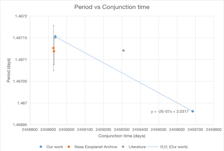
Figure 15. The graph drawn in the data table (The width of this work’s error bar is approximately one tenth of that of other researchers).

There could be some unknown natural slight factors that are consistently affecting the orbital period. For example, there might be a non-transiting planet in the same planetary system that constantly affects the observational subject with its gravitational influence. After predicting and calculating dp/dt based on known data and relevant formula, this work finds that evident difference exists between the estimation and result, and roughly guesses the two kinds of potential causes. Some further research will be done on this difference in the future, but before that this work will have to reassure its error boundaries and make it more precise---might be some new information revealed.

6. Conclusion

Many other groups of researchers have finished their investigation on GJ 486, using various methods. The results from best-fit models are generally the same, while the range of error bars and results of some further analysis is different. For now, the credibility of the results remains undetermined, as some important factors lie unknown and the related data is scarce---as the planet is not discovered until 2020. Meanwhile, some formula researchers have to use cannot make theoretical prediction precisely. Owing to things above, potential directions for future study involves developing more equations with present theory and figuring out means to determine more parameters that crucial for further analysis like the stellar and planetary tidal quality factor. More importantly, researchers can make similar investigation on the “young” exoplanet, hunting for unexpected changes and more accurate results, as the universe is broad and mysterious, where unnumbered unknowns lie.

References

[1]. Trifonov, T., (2021) A nearby transiting rocky exoplanet that is suitable for atmospheric investigation. Science 371, 1038–1041
[2]. Smith, K. T. . (2021). A transiting rocky planet 8 parsecs away. Science(6533).
[3]. Mandel, K., Agol, E. (2002) Analytic Light Curves for Planetary Transit Searches. Astrophys. J. 580, L171-L175
[4]. Claret A., 2018, Limb-darkening for TESS, Kepler, Corot, MOST http://cdsarc.u-strasbg.fr/viz-bin/nph-Cat/html?J/A+A/618/A20/table5.dat
[5]. José A. Caballero, 2022. A detailed analysis of the Gl 486 planetary system. https://arxiv.org/abs/2206.09990.
[6]. Claret, A. (2018). A new method to compute limb-darkening coefficients for stellar atmosphere models with spherical symmetry: the space missions TESS, Kepler, CoRoT, and MOST . Astronomy & Astrophysics, 618, A20.
[7]. Astropy. Box Least Squares (BLS) Periodogram. https://docs.astropy.org/en/stable/timeseries/bls.html Kurtz, D. W. (2022). Asteroseismology Across the Hertzsprung–Russell Diagram. Annual Review of Astronomy and Astrophysics, 60(1).
[8]. Kurtz, D. W. (2022). Asteroseismology Across the Hertzsprung–Russell Diagram. Annual Review of Astronomy and Astrophysics, 60(1).
[9]. Stello, D., Saunders, N., Grunblatt, S., Hon, M., Reyes, C., Huber, D., Bedding, T. R., Elsworth, Y., García, R. A., Hekker, S., Kallinger, T., Mathur, S., Mosser, B., & Pinsonneault, M. H. (2022). TESS asteroseismology of the Kepler red giants. Monthly Notices of the Royal Astronomical Society, 512(2), 1677–1686.
[10]. Brady, M. T., & Bean, J. L. (2022). Assessing the Transiting Exoplanet Survey Satellite’s Yield of Rocky Planets Around Nearby M Dwarfs. The Astronomical Journal, 163(6), 255.
[11]. Patra, K. C. , Winn, J. N. , Holman, M. J. , Gillon, M. , & Broome, M. . (2020). The continuing search for evidence of tidal orbital decay of hot jupiters. The Astronomical Journal, 159(4), 150.
Cite this article
Zhou,Z.;Li,J.;Zhong,Y.;Hou,Z.;Yao,R. (2023). Analysis on Gliese 486 b. Theoretical and Natural Science,5,734-749.
Data availability
The datasets used and/or analyzed during the current study will be available from the authors upon reasonable request.
Disclaimer/Publisher's Note
The statements, opinions and data contained in all publications are solely those of the individual author(s) and contributor(s) and not of EWA Publishing and/or the editor(s). EWA Publishing and/or the editor(s) disclaim responsibility for any injury to people or property resulting from any ideas, methods, instructions or products referred to in the content.
About volume
Volume title: Proceedings of the 2nd International Conference on Computing Innovation and Applied Physics (CONF-CIAP 2023)
© 2024 by the author(s). Licensee EWA Publishing, Oxford, UK. This article is an open access article distributed under the terms and
conditions of the Creative Commons Attribution (CC BY) license. Authors who
publish this series agree to the following terms:
1. Authors retain copyright and grant the series right of first publication with the work simultaneously licensed under a Creative Commons
Attribution License that allows others to share the work with an acknowledgment of the work's authorship and initial publication in this
series.
2. Authors are able to enter into separate, additional contractual arrangements for the non-exclusive distribution of the series's published
version of the work (e.g., post it to an institutional repository or publish it in a book), with an acknowledgment of its initial
publication in this series.
3. Authors are permitted and encouraged to post their work online (e.g., in institutional repositories or on their website) prior to and
during the submission process, as it can lead to productive exchanges, as well as earlier and greater citation of published work (See
Open access policy for details).