


1. Introduction
Astrophysicists have found several evidence for the existence of dark matters through the observation of different astrophysical sources from cluster of galaxies up to individual galaxies [1].
In particular, one of the first evidence for the existence of dark matter is related to the estimation of the mass of the Coma cluster. The mass of this object can be estimated using the luminosity produced by the galaxies in the cluster. This gives an estimate of the so-called luminous mass, which is related to the mass of baryons. However, this is not the same of the gravitational mass, which is the actual total mass of the system. According to the Virial Theorem, the kinetic energy of a system of particles (K) is related to the gravitational potential energy (U) as: \( K=U/2 \) . By further expanding this expression, the theoretical mass, which is the gravitational mass of the object, should be calculated by: \( M={v^{2}}R/G \) . The viral theorem can thus be used to calculate the real mass of the cluster including baryonic and non-baryonic matter. However, in reality, the visible mass, associated to stars and gas, is much smaller than the gravitational mass, indicating there might be a large amount of “dark mass”. In the Coma cluster in particular the baryonic matter is only a few % of the total one. This dark mass, which could be make of dark matter particles, makes the 85% of the total matter in the Universe and drives most of the gravitational forces that keep together astrophysical sources.
Vera Rubin and collaborators verified the existence of dark matter by observing the rotational velocity of stars in the Andromeda Galaxy [2]. Through these observations, Vera Rubin and her colleagues successfully determined the rotation curve of the galaxy. Theoretically, the rotational velocity of stars should be given by \( v(r)=\sqrt[]{GM(r)/r} \) . Considering the typical dependence of star and gas mass with radius, the velocity should be inversely proportional to the radius of the position to the power of, meaning the velocity will get smaller as the radius increases. However, according to the observed curve found by Vera Rubin and collaborators, the rotational velocity data are flat for distance beyond 10 kpc from the center of the galaxy, which means the velocities of the stars in the outer spirals are almost the same as the stars in the inner spirals. This conclusion, confirmed in several other observations, indicates that there is a massive invisible dark matter which is very abundant in galaxies and that drives most of the gravitational force in the outer regions. In particular, the dark matter halo present in most of the galaxies is spherically symmetric and has an extent of 100-200 kpc. Moreover, since the velocity is flat with radius the density of dark matter should be proportional to the radius to the power of -2.
Gravitational lensing also provides powerful evidence of dark matter. Albert Einstein predicted that strong mass could bend the light from other sources towards themselves. By observing the lensing effect of known cosmic objects, scientists found out that the distortion of light is far too much for the known mass. Therefore, there must be some invisible masses helping bend more light.
The goal of this paper is to review recent data and models relevant to find the dark matter density in the Milky Way. We will use two methods to determine the dark matter density parameter. One that uses only the information of the local dark matter density and total dark matter mass. The second, which is also more precise, take into account the rotation curve velocity of the Milky Way as a function of radius. By properly including the bulge and disk components as well as the dark matter halo contribution we will be finding the density of the latter.
The paper is organized as follow: part 2 contains the data for the rotational velocities of the Milky Way Galaxy (i.e. the velocity curve of the central bulge and the disk) and current methods of measuring the rotational curve, part 3 explains our estimation of the dark matter density profile using the total dark matter mass and local dark matter density, part 4 is the analysis of the plot of the real rotational curve of Milky Way Galaxy and thus leading to the discussion of the density distribution of dark matter in the galaxy, part 5 contains the summary for this work.
2. Rotational curve of the milky way
2.1. Current methods of measuring rotational curves
In this section we report the main methods to measure the velocity of star in galaxies.
2.1.1. Tangent point method. The Tangent Point Method is a commonly used method to determine the rotational curve of the inner portion Milky Way. It is based on the assumption that along one line of sight, the point tangent to the Galactic center is the point where the observed radial velocity is an extremum [3]. Then the velocity V(R) of the galaxy at the location of R can be simply derived by the observed radial velocity by basic trigonometry.
2.1.2. Radial-velocity+distance method. The distance of celestial body can be measured through spectroscopic and/or trigonometric observations. The radial velocity can be found by the observed Doppler shift, in particular, red shift, of the spectral line. By geometric conversion of radial velocity, distance and the longitude of the observer, the rotational velocity can be resolved.
2.1.3. Trigonometric method. If the radial velocity and distance of a certain source is measured by observers at different locations and the same time, the 3D velocity vector of this source can be determined, and hence the rotational velocity can be solved.
2.1.4. Disk-thickness method. The method is to use the variation with galactic longitude in the angular thickness of the HI disk and the HI data cube to find the distance of certain slice [4].
2.2. Unified rotational curve
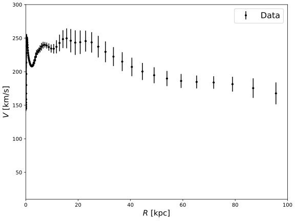
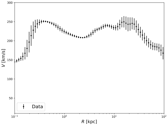
The data for unified rotational curve in this paper is adopted by averaging formerly done work [5]. In particular in that reference the author took available data from different observations and averaged over them. The plotted curve is shown in Figure 1 as in linear scale and logarithm scale. The scale of the radius is from 0.1 to 95.56 kpc. The error bars come from standard deviations within each Gaussian-averaging bin.
As indicated in Figure 1, the rational velocity of Milky Way increases significantly from 0.1 to 0.5 kpc from the center of the Galaxy until it reaches the maximum, and then decreases from that position until the edge of the bulge, which is about 2-3 kpc from the center. As reaching to the galactic disk, the rotational velocity again increases until 20 kpc form the center, and then gradually decreases from that point until the edge of the galactic disk.
|
| |
Figure 1. Unified observed rotational curve of Milky Way in Linear scale (left panel) and logarithmic scale (right panel). Data are taken from3. | ||
2.3. Mass distribution
The Milky Way is composed by the central black hole and star bulge, the disk and dark matter. All these components are important and should be taken into account to have a correct prediction of the rotational velocity. In particular, in the inner parsec region the supermassive black hole present in the center of the Galaxy can play a role. Instead inside a few kpc the star bulge plays the most important role. In the intermediate regions the star and gas components present in the disk are the dominant contributor to the velocities. Finally, for distances larger than 10 kpc the dark matter component is the dominant one. Since, the data we have are taken for distances from the Galactic center much larger than the parsec scale, we neglect the supermassive black hole in the center of the Milky Way since this is not going to play any role in the interpretation of the data.
2.3.1. De Vaucouleurs Bulge. The Galactic bulge represents the inner density and population of stars present in the Milky Way. This is the densest region for the star population in the Galaxy which is constituted by an old population that fell in the center of the Galaxy due to gravity acting for millions of years.
To integrate the mass for the central bulge, the most commonly used method is to find the surface mass density first and then relate the volume mass density with it. The surface mass density (SMD) of the central bulge is assumed to be proportional to the empirical optical profile of the surface brightness. By de Vaucouleurs law[6]:
\( \sum _{b}(R)=\sum _{be}exp[-7.6695({(\frac{R}{{R_{b}}})^{\frac{1}{4}}}-1)]\ \ \ (1) \)
\( {Σ_{be}} \) represents the the value at radius enclosing a half of the integrated surface mass.
The volume mass density for the central bulge is related to the SMD by the following expression:
\( ρ(r)=\frac{1}{π}\int _{r}^{∞}\frac{d{Σ_{b}}(x)}{dx}\frac{1}{\sqrt[]{{x^{2}}-{r^{2}}}}dx\ \ \ (2) \)
Then the mass of the central bulge can be calculated by direct integration:
\( dM=ρ(r)\cdot dV=ρ(r)\cdot 4π{r^{2}}dr\ \ \ (3) \)
\( M=\int _{0}^{R}dM=4π\int _{0}^{R}{r^{2}}ρ(r)dr\ \ \ (4) \)
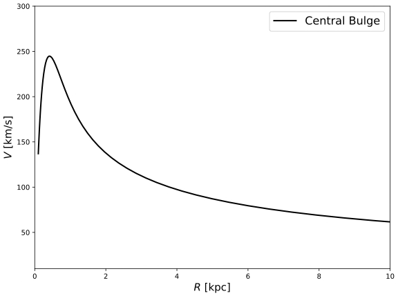
The velocity of the bulge is related to the mass by the equation for centripetal force and the gravitational force:
\( \frac{GM(R)m}{R}=\frac{mV_{b}^{2}}{R}{⟹V_{b}}(R)=\sqrt[]{\frac{GM(R)}{R}}\ \ \ (5) \)
In Figure 2 we show the plot for rotational curve for the central bulge within the interval of 0 kpc \( ≤ \) R \( ≤ \) 10 kpc. We see from the figure that the bulge has a peak at around 0.5 kpc where it provides the largest contribution. Instead, for radii larger than a few kpc this component does not contribute significantly to the velocity.
| Figure 2. Rotational Curve velocity given by the Central Bulge stars. |
2.3.2. Galatic disk. In addition to the Galactic bulge, that is most relevant for inner few kpc, younger stars populate the Galaxy in the spiral arms which are located in the disk. In the disk, together with stars also gas makes an important fraction of the total Milky Way mass and should be thus taken into account. The mass of the Galactic disk is calculated directly through surface mass density of the disk by the expression [7]:
\( {M_{disk}}=2π{Σ_{dc}}R_{d}^{2}\ \ \ (6). \)
The SMD for the disk is often expressed in the form of an exponential disk:
\( \sum _{d}R=\sum _{d}exp(-\frac{R}{{R_{d}}})\ \ \ (7) \) .
The velocity for an exponential disk with infinitesimal thickness is expressed by:
\( {V_{d}}(R)=\sqrt[]{4πG{Σ_{0}}{R_{d}}{y^{2}}[{I_{0}}(y){K_{0}}(y)-{I_{1}}(y){K_{1}}(y)]}\ \ \ (8). \)
In the expression, \( y=R/(2{R_{d}}) \) , \( {I_{i}} \) and \( {K_{i}} \) are modified Bessel functions.
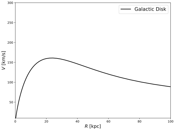
Figure 3 and 4 are the plots for RC for the Galactic disk within the interval of 0 kpc \( ≤ \) R \( ≤ \) 100 kpc. The figure shows that the disk component has a bump shape with a peak at around 20 kpc, which is the typical radius of the Milky Way disk. Instead, at larger radii the velocity decreases and thus this component is going to contribute much less to the total velocity.
| Figure 3. Rotational Curve of the Galactic Disk. |
2.3.3. Theoretical RC without DM. Combining the rotational curve of the central bulge and the Galactic disk, we can obtain a predicted rotational curve of the Milky Way Galaxy presuming only baryonic substances exist. The combined curve is the presented by the grey curve in Figure 4:
| Figure 4. Theoretical RC without DM [Linear]. |
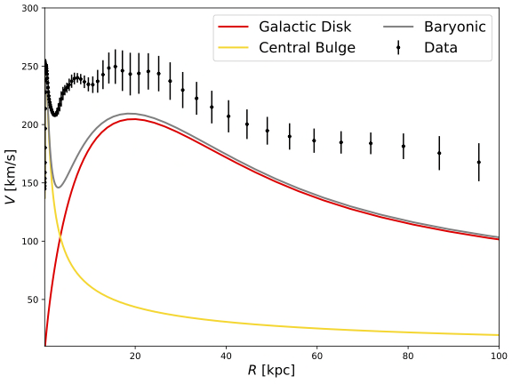
As Figure 4 shows, there is a huge gap between the theoretical rotational curve of only visible matters and the observed rotational curve. This indicates the existence of dark matter in the galaxy.
3. Dark halo
3.1. Dark matter profiles
Several models for dark matter profiles had been proposed, and the unification of these profiles has not been reached. Therefore, this work will discuss 6 different models: Navarro-Frenk-White, Einasto, Burkert, Isothermal and Moore model. Their density profiles are reported below:
NFW model:
\( {ρ_{NFW}}(r)={ρ_{s}}\frac{{r_{s}}}{r}(1+\frac{r}{{r_{s}}}{)^{-2}} \) (9)
Einasto model:
\( {ρ_{Ein}}(r)={ρ_{s}}exp\lbrace -\frac{2}{α}[(\frac{r}{{r_{s}}}{)^{α}}-1]\rbrace \) (10)
Burkert model:
\( {ρ_{Bur}}(r)=\frac{{ρ_{s}}}{(1+r/{r_{s}})(1+(r/{r_{s}}{)^{2}})} \) (11)
Isothermal model:
\( {ρ_{Iso}}(r)=\frac{{ρ_{s}}}{1+(r/{r_{s}}{)^{2}}} \) . (12)
Moore model:
\( {ρ_{Moo}}(r)={ρ_{s}}(\frac{{r_{s}}}{r}{)^{1.16}}(1+\frac{r}{{r_{s}}}{)^{-1.84}} \) . (13)
In each of the above-mentioned density profiles there are two parameters that must be found. The first one is \( {ρ_{s}} \) which represents a normalisation factor and the second is \( {r_{s}} \) and it is a scale radius at which the density profile typically change slope.
In order to plot the rotational curve of Dark Matter, the parameters (i.e. \( {r_{s}} \) , a typical scale radius and \( {ρ_{s}} \) , a typical scale density) in each of the above profiles shall be determined.
To determine the parameters, we impose some known astrophysical observations into the expression:
• The total Dark Matter mass contained within 60 kpc relative to the centre of the Milky Way is \( {M_{60}}≡4.659×{10^{11}}{M_{⊙}} \) . This is from a recent kinematical survey of stars in 2008 by SDSS [8].
• The Dark Matter density located near the Sun is 0.3 GeV/cm3. This is a commonly accepted value routinely adopted in Dark Matter related articles. The error bar of this value is debatable. The possible spread is 0.1-0.8 GeV/cm3. Here in this article, we adopt the value of 0.35 GeV/cm3.
• The location of the Sun within the Milky Way is: \( {r_{⊙}}=8.33 \) kpc [9].
Below we report the demonstration of how to solve for \( {r_{s}} \) and \( {ρ_{s}} \) with the NFW profile. The method shall be adopted by all profiles mentioned earlier in this section. All computations involved were done via python.
By inputting the location of the Sun into the NFW equation and temporarily setting the value of \( {ρ_{s}} \) as 1, we can set a new variable for computation convenience, “density”, which is a function with only a single unknown variable \( {r_{s}} \) :
\( ρ \) (1, \( {r_{s}} \) , \( {r_{local}} \) ) = \( \frac{{r_{s}}}{{r_{l}}}(1+\frac{{r_{l}}}{{r_{s}}}{)^{-2}} \) = \( \frac{{ρ_{NFW}}}{{ρ_{s}}} \) . (14)
As previously stated, the commonly accepted Dark Matter density value near the location is \( {ρ_{local}} \) = 0.35 GeV/cm3. By inputting this value:
\( {ρ_{s}}={ρ_{local}}\cdot (\frac{{r_{s}}}{{r_{l}}}(1+\frac{{r_{l}}}{{r_{s}}}{)^{-2}}{)^{-1}} \) . (15)
Here we successfully transferred \( {ρ_{s}} \) as a function of \( {r_{s}} \) . To further use the observed total Dark Matter mass contained within 60 kpc, \( {M_{60}} \) , we need to set up an equation connecting \( {r_{s}} \) with \( {M_{60}} \) .
\( {M_{60}}=∫_{60}^{0}4π{ρ_{NFW}}{r^{2}}≡4.659×{10^{11}}{M_{⊙}} \) . (16)
In the above equation, the only unknown variable is \( {r_{s}} \) (since \( {ρ_{s}} \) had already been transferred into a function of \( {r_{s}} \) in the previous steps). Hence the value of \( {r_{s}} \) and \( {ρ_{s}} \) can be easily solved.
Below is the table of parameters fit by each profile.
Table 1. Parameters for different DM profiles. | ||
DM Profile | \( {r_{s}} \) [kpc] | \( {ρ_{s}} \) [kpc] |
NFW | 18.28 | 0.34 |
Einasto | 18.71 | 0.08 |
Isothermal | 0.92 | 29.03 |
Burkert | 11.06 | 0.96 |
Moore | 21.93 | 0.70 |
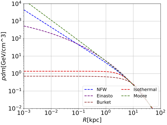
Plugging in the above parameters to the DM profiles, we obtain the plot showing the Dark Matter behaviour according to different profiles. In particular, we can see that the Isothermal and Burkert profilers are flat for large distances from the Galactic center. In fact, these functional forms are labeled as cored profiles. Instead, the NFW, Moore and Einasto are steeper in the inner region, and they are typically called cusp profiles. All the density profiles have the same value at the local distance from the Galactic center because this is a condition we applied in our method. The values we find are very similar with the ones found in this paper [10].
| Figure 5. Galactic Distribution of Dark Matter through different DM profiles. |
3.2. Rotational curve of dark matter
In this paper, the rotational curve of dark matter halo in the Milky Way galaxy is obtained in two different DM density profiles proposed by former works, NFW[11] and Burkert[12].
NFW model:
\( {ρ_{NFW}}(r)={ρ_{s}}\frac{{r_{s}}}{r}(1+\frac{r}{{r_{s}}}{)^{-2}} \) . (17)
Burkert model:
\( {ρ_{Bur}}(r)=\frac{{ρ_{s}}}{(1+r/{r_{s}})(1+(r/{r_{s}}{)^{2}})} \) . (18)
The parameters of normalization factor ( \( {ρ_{s}} \) ) and scale radius ( \( {r_{s}} \) ) of the above two profiles have been found in part 2 in this paper.
From the density profiles, the mass function of local dark matter halo with respect to the location is determined by:
\( M=∫_{0}^{R}dM=4π∫_{0}^{R}{r^{2}}ρ(r)dr \) . (19)
Then by the equation for centripetal force and the gravitational force: \( {V_{DM}}(R)=\sqrt[]{\frac{GM(R)}{R}} \) .
Below are the rational curves of dark matter halos:
|
| |
Figure 6. RC of the DM Halo by NFW profile [Logarithmic scale]. | Figure 7. RC of the DM Halo by NFW profile [Linear scale]. | |
|
| |
Figure 8. RC of the DM Halo by Burkert profile [Logarithmic scale]. | Figure 9. RC of the DM Halo by Burkert profile [Linear scale]. |
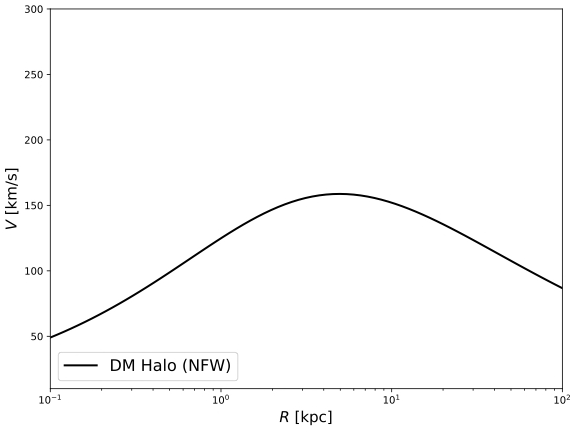
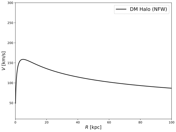
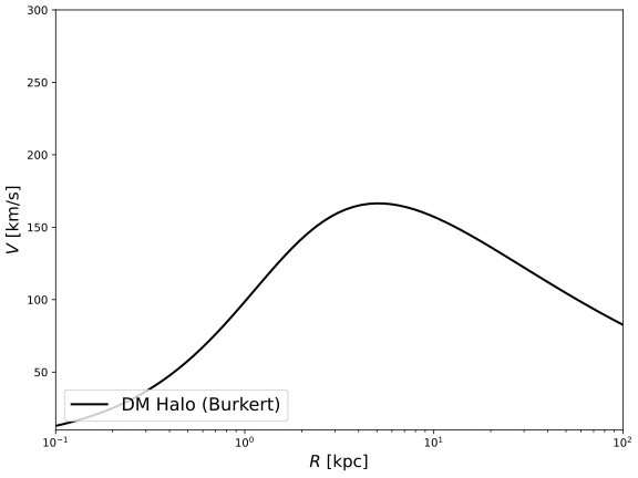
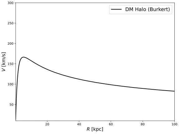
As the above four figures show, in the linear scale, both NFW and Burkert profiles generally give out similar characteristics of the density of DM with respect to the location, which is increase rapidly from the center of the galaxy until about 3 kpc from the center, which is near the edge of the central bulge, and then gradually decrease at a decreasing rate. This indicates that the density of dark matter achieves a maximum at the edge of the central bulge and then gradually decrease along the galactic disk. In the log scale, on the other hand, the NFW profile indicates the existence of dark matter halo in the center of the galaxy, while the Burkert profile stands the point that there is almost no existence of dark matter at the center of the galaxy.
4. DM density by fitting observed RC of the galaxy
The composite rotational velocity of the milky way galaxy is obtained by the square root of the square sum of three mass components — central bulge, galactic disk and dark matter:
\( {V_{tot}}=[({V_{b}}{)^{2}}+({V_{d}}{)^{2}}+({V_{DM}}{)^{2}}{]^{\frac{1}{2}}} \) . (20)
The \( {r_{s}} \) values for Burkert and NFW profile optimized from the rotational curves are:
NFW:
\( {r_{s}}=2.287 \)
Burkert:
\( {r_{s}}=1.567 \)
In each of the below figures, the composite RC of the galaxy is represented by the grey curve.
|
| |||||
Figure 10. Composite RC of the Milky Way galaxy by NFW DM profile [Linear scale]. | Figure 11. Composite RC of the Milky Way galaxy by NFW DM profile [Logarithmic scale]. | |||||
|
| |||||
Figure 12. Composite RC of the Milky Way galaxy by Burkert DM profile [Linear scale]. | Figure 13. Composite RC of the Milky Way galaxy by Burkert DM profile [Logarithmic scale]. | |||||
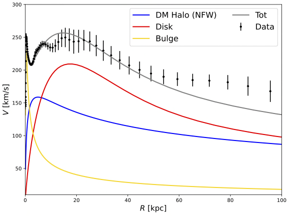
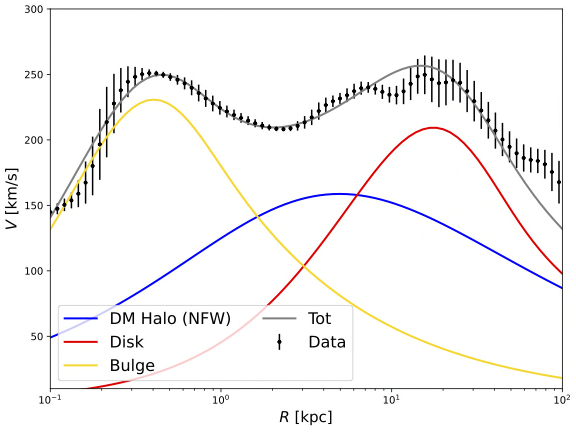
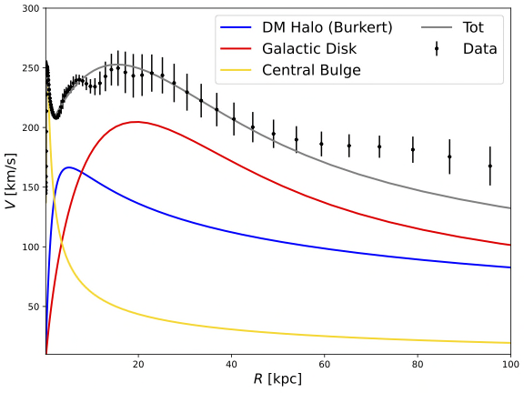
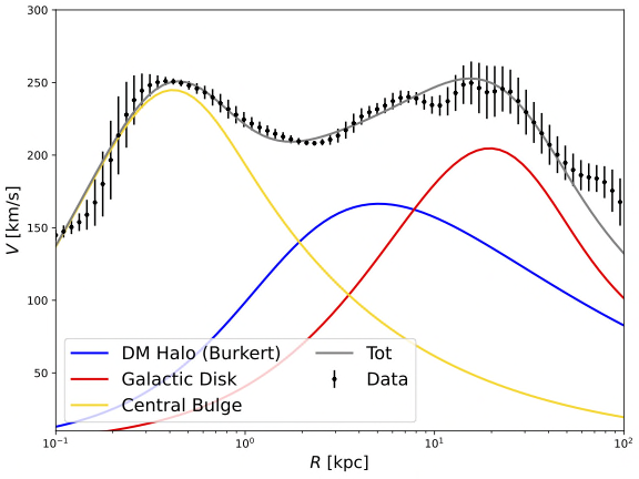
The composite curve falls within the error bars of each point, indicating a good fit. According to Figure 9-12, Both NFW and Burkert profile give similar characteristics. From the center of the galaxy (R = 0 kpc) to about the edge of the central bulge (R = 2-3 kpc), the central bulge contributes the most to the rotational velocity. Then the dominant component becomes the dark matter halo from the edge of the bulge (2-3 kpc) until about 10 kpc. Starting from R = 10 kpc, the baryonic objects in the galactic disk become the dominant component of the rotational velocity until the edge of the Milky Way galaxy.
In particular, the dark halo density reaches the maximum at about 8 kpc from the galaxy center in both NFW and Burkert profiles. This is significant since the solar system locates exactly at about 8 kpc from the center of the galaxy. This suggests that the location of the Earth might happen to be an optimal position to further study the nature of black matters.
5. Conclusion
In this paper, we reviewed the recent retrieved data regarding the Rotation Curve of the Milky Way galaxy. By these formerly presented data, we decomposed the constituents of the Galaxy into the central bulge, Galactic disk and dark halo, and then generated a unified rotational curve. By the generated unified rotational curve, the density distribution of dark matter halo in the Milky Way Galaxy shall be reflected. According to the outcome of the model, the dark matter halo has a dominant density within the range 2 kpc < R < 10 kpc, and our solar system happens to locate within this range.
References
[1]. Bertone, G., Hooper, D., & Silk, J. (2005). Particle dark matter: Evidence, candidates and constraints. Physics Reports, 405(5-6), 279–390. https://doi.org/10.1016/j.physrep.2004.08.031
[2]. Rubin, V. C., & Ford, W. K. (1970). Rotation of the andromeda nebula from a spectroscopic survey of emission regions. The Astrophysical Journal, 159, 379. https://doi.org/10.1086/150317
[3]. Chiu CK, Strigari LE. Testing the accuracy of the tangent point method for determining the Milky Way’s inner rotation curve. Research notes of the AAS. 2020;4(9):165. http://dx.doi.org/10.3847/2515-5172/abbad8. doi:10.3847/2515-5172/abbad8
[4]. Merrifield, Michael R. "The rotation curve of the Milky Way to 2.5 R0 from the thickness of the HI layer." The Astronomical Journal 103 (1992): 1552-1563.
[5]. Sofue, Y. Rotation and mass in the Milky Way and spiral galaxies. Publ. Astron. Soc. Jpn. 2017, 69, R1
[6]. Vaucouleurs, G. (1948). Annales d'Astrophysique, Vol. 11, p. 247.
[7]. Chabrier, G. (2003). The galactic disk mass function: Reconciliation of the [ital]hubble space telescope[/ital] and nearby determinations. The Astrophysical Journal, 586(2). https://doi.org/10.1086/374879
[8]. X. X. Xue et al. [SDSS Collaboration], As- trophys. J. 684 (2008) 1143 [arXiv:0801.1232 [astro-ph]]
[9]. S. Gillessen, F. Eisenhauer, S. Trippe, T. Alexander, R. Genzel, F. Martins and T. Ott, Astrophys. J. 692 (2009) 1075 [arXiv:0810.4674 [astro-ph]]
[10]. Cirelli, M., Corcella, G., Hektor, A., Hütsi, G., Kadastik, M., Panci, P., Raidal, M., Sala, F., & Strumia, A. (2012). Erratum: PPPC 4 DM ID: A poor particle physicist cookbook for dark matter indirect detection. Journal of Cosmology and Astroparticle Physics, 2012(10). https://doi.org/10.1088/1475-7516/2012/10/e01
[11]. J. F. Navarro, C. S. Frenk and S. D. M. White, Astrophys. J. 462 (1996) 563 [arXiv:astro- ph/9508025].
[12]. A. Burkert, IAU Symp. 171 (1996) 175 [Astrophys. J. 447 (1995) L25] [arXiv:astro- ph/9504041].
Cite this article
He,Y. (2023). Updated estimate for the dark matter density in the milky way. Theoretical and Natural Science,12,202-211.
Data availability
The datasets used and/or analyzed during the current study will be available from the authors upon reasonable request.
Disclaimer/Publisher's Note
The statements, opinions and data contained in all publications are solely those of the individual author(s) and contributor(s) and not of EWA Publishing and/or the editor(s). EWA Publishing and/or the editor(s) disclaim responsibility for any injury to people or property resulting from any ideas, methods, instructions or products referred to in the content.
About volume
Volume title: Proceedings of the 2023 International Conference on Mathematical Physics and Computational Simulation
© 2024 by the author(s). Licensee EWA Publishing, Oxford, UK. This article is an open access article distributed under the terms and
conditions of the Creative Commons Attribution (CC BY) license. Authors who
publish this series agree to the following terms:
1. Authors retain copyright and grant the series right of first publication with the work simultaneously licensed under a Creative Commons
Attribution License that allows others to share the work with an acknowledgment of the work's authorship and initial publication in this
series.
2. Authors are able to enter into separate, additional contractual arrangements for the non-exclusive distribution of the series's published
version of the work (e.g., post it to an institutional repository or publish it in a book), with an acknowledgment of its initial
publication in this series.
3. Authors are permitted and encouraged to post their work online (e.g., in institutional repositories or on their website) prior to and
during the submission process, as it can lead to productive exchanges, as well as earlier and greater citation of published work (See
Open access policy for details).
References
[1]. Bertone, G., Hooper, D., & Silk, J. (2005). Particle dark matter: Evidence, candidates and constraints. Physics Reports, 405(5-6), 279–390. https://doi.org/10.1016/j.physrep.2004.08.031
[2]. Rubin, V. C., & Ford, W. K. (1970). Rotation of the andromeda nebula from a spectroscopic survey of emission regions. The Astrophysical Journal, 159, 379. https://doi.org/10.1086/150317
[3]. Chiu CK, Strigari LE. Testing the accuracy of the tangent point method for determining the Milky Way’s inner rotation curve. Research notes of the AAS. 2020;4(9):165. http://dx.doi.org/10.3847/2515-5172/abbad8. doi:10.3847/2515-5172/abbad8
[4]. Merrifield, Michael R. "The rotation curve of the Milky Way to 2.5 R0 from the thickness of the HI layer." The Astronomical Journal 103 (1992): 1552-1563.
[5]. Sofue, Y. Rotation and mass in the Milky Way and spiral galaxies. Publ. Astron. Soc. Jpn. 2017, 69, R1
[6]. Vaucouleurs, G. (1948). Annales d'Astrophysique, Vol. 11, p. 247.
[7]. Chabrier, G. (2003). The galactic disk mass function: Reconciliation of the [ital]hubble space telescope[/ital] and nearby determinations. The Astrophysical Journal, 586(2). https://doi.org/10.1086/374879
[8]. X. X. Xue et al. [SDSS Collaboration], As- trophys. J. 684 (2008) 1143 [arXiv:0801.1232 [astro-ph]]
[9]. S. Gillessen, F. Eisenhauer, S. Trippe, T. Alexander, R. Genzel, F. Martins and T. Ott, Astrophys. J. 692 (2009) 1075 [arXiv:0810.4674 [astro-ph]]
[10]. Cirelli, M., Corcella, G., Hektor, A., Hütsi, G., Kadastik, M., Panci, P., Raidal, M., Sala, F., & Strumia, A. (2012). Erratum: PPPC 4 DM ID: A poor particle physicist cookbook for dark matter indirect detection. Journal of Cosmology and Astroparticle Physics, 2012(10). https://doi.org/10.1088/1475-7516/2012/10/e01
[11]. J. F. Navarro, C. S. Frenk and S. D. M. White, Astrophys. J. 462 (1996) 563 [arXiv:astro- ph/9508025].
[12]. A. Burkert, IAU Symp. 171 (1996) 175 [Astrophys. J. 447 (1995) L25] [arXiv:astro- ph/9504041].