1. Introduction

Situated along the main course of the Colorado River, Lake Mead holds the distinction of being the largest reservoir in the entire United States when at full capacity. Nestled approximately 30 miles east of Las Vegas, within the arid Mojave Desert spanning both Arizona and Nevada, Lake Mead stretches an impressive 65 miles from Hoover Dam to Pearce Ferry, attaining a maximum width of 9.3 miles. This vast reservoir boasts a staggering current-related capacity of 2,998,000 horsepower and provides essential daily water supplies to approximately 25,000,000 people in the surrounding regions.

However, Lake Mead is currently grappling with a severe issue of aridity. The Upper Basin endured an exceptionally dry spring in 2021, resulting in runoff into Lake Powell amounting to only \( 26\% \) of the long-term average, despite receiving near-average snowfall in the preceding winter. The projected unregulated inflow into Lake Powell for the water year 2021, which represents the natural flow into Lake Mead without the influence of reservoir storage behind Glen Canyon Dam, is estimated to be a mere \( 32\% \) of the long-term average [1]. Consequently, the storage levels of the entire Colorado River system have plummeted to a mere \( 40\% \) of their total capacity, marking a significant decline from the previous year's level of \( 49\% \) . This decline can be attributed to the reduced inflow from the primary water sources. Moreover, since 1999, the population residing in the vicinity of the lake has steadily increased, leading to a corresponding surge in water demand. The burgeoning demand for water resources has further exacerbated the shortage crisis.

To effectively address the pressing issue of drought at Lake Mead, it is imperative to develop mathematical models capable of solving the following critical problems:

Explore the factors influencing Mead Lake's inflow, outflow, and water loss while examining their interrelationships and their impact on water levels.

Gather additional data to create a lake bottom model and investigate the correlation between specific depths and overall volume.

Establish criteria for defining dry periods at Lake Mead, and then compare the ongoing dry spell with past occurrences.

Develop a water level prediction model utilizing both short-term and long-term data to forecast Lake Mead's water levels in 2025, 2030, and 2050. Subsequently, compare and assess the outcomes of the two models.

Conduct research on a wastewater recycling plan, prioritize various factors, and gauge the plan's impact.

Summarize research findings in a non-technical news brief. Provide concise summaries of research conclusions and recommendations.

2. General Assumptions and Notations

2.1. General Assumptions

To simplify the problem and facilitate the simulation of practical conditions, the following basic assumptions are made, and their accuracy is meticulously evaluated.

Steady Water Demand: Assumptions are made that the water demand of the populace remains constant, regardless of the water supply. In other words, people's water consumption remains unchanged and can be precisely calculated [2].

Zero Water Loss during Transportation: It is assumed that Lake Mead does not experience any water loss during the process of supplying water to the city. This implies that there is no water loss during transportation.

Negligible Water Infiltration: For the purposes of this study, water infiltration is not considered a factor. In other words, the paper does not account for any loss of water due to infiltration.

2.2. Notations

Throughout the paper, it can be seen as follows

Table 1. Notations.

In this section, only the main parameters are defined, with the remaining parameters provided in the subsequent paper.

3. Establishment of the Water Volume Model of Lake Mead

3.1. Factors related to the water volume of Lake Mead

The water volume of Lake Mead is influenced by three primary factors: water inflow, water outflow, and water loss. This relationship can be expressed through the following formula:

\( C=L-O-W\ \ \ (1) \)

Here, C represents the change in water volume (an increase is denoted as a positive number). L signifies the inflow water volume, O is the outflow water volume, and W represents water volume loss.

The current water volume can be determined by adding the water volume change to the existing water volume:

\( V=S+C\ \ \ (2) \)

In this equation, V stands for the existing water volume, and S is the previous water volume.

The factors affecting water inflow include the influx of water from its sources. On the other hand, the factors influencing water outflow consist of dam discharge in response to precipitation, while residential water consumption contributes to water loss primarily through evaporation.

3.2. Inflow

3.2.1. Direct inflow. Most of Lake Mead's water inflow is derived from connected rivers, primarily the Colorado River, which accounts for approximately 90% of the total inflow. The Colorado River originates in the western Rocky Mountains, primarily fueled by melting snow [3]. It courses through several states, including Wyoming, Colorado, Utah, New Mexico, Nevada, Arizona, and California, before ultimately merging into the Gulf of California. The Colorado River spans 1,450 miles, boasts an average flow of 620 cubic meters per second, and covers a drainage area of 63,700 square meters [4]. Notably, Lake Mead is directly connected to the Colorado River, effectively capturing its entire flow. This standard can also be applied to the other three tributaries. Based on the proportion of the Colorado River's flow indicated in the available data, the daily inflow can be directly calculated using the following formula:

\( ΣL=({L_{k}}+{L_{r}})×86400\ \ \ (3) \)

Where \( ΣL \) represents daily inflow, \( {L_{k}} \) is the average flow of the Colorado River, and \( {L_{r}} \) represents flow Using the provided data as an example:

\( ΣL=(620+620×\frac{4}{96})×86400=5.58×{10^{7}}(cubic meter per day)\ \ \ (4) \)

3.2.2. Precipitation inflow. On the flip side, direct precipitation also contributes to approximately 10% of Lake Mead's inflow. The average annual precipitation at Lake Mead varies between 100ml and 400ml, with this year experiencing a particularly low point of 100ml due to the western drought. We can estimate the annual precipitation either within this range or based on the average annual precipitation for a specific year. To determine the amount of water collected by Lake Mead from precipitation, we consider only the water that directly falls onto the lake's surface. This can be calculated as follows:

\( {L_{d}}=\frac{{L_{y}}×S}{365}\ \ \ (5) \)

Here, \( {L_{d}} \) represents daily precipition collection, \( {L_{y}} \) stands for average annual precipitation, and S is the surface area of Lake Mead. Using this year's data as an example, with an annual precipitation of 100 \( ml/m³ \) and a Lake Mead area of 593 \( km² \) , we can calculate:

\( {L_{d}}=\frac{100×593}{365}≈1.62×{10^{6}}(cubic meters per day)\ \ \ (6) \)

This calculation highlights how the western U.S. drought this year significantly affected Lake Mead's precipitation inflow.

Although Lake Mead is situated in the western United States and is relatively close to the Pacific Ocean, the presence of substantial mountain ranges surrounding it restricts the influx of water vapor. Consequently, the impact of water vapour condensation on Lake Mead is negligible [5].

When we sum up the total inflow, considering both water sources (approximately \( 5.58×{10^{7}}+1.6×{10^{6}} \) ), the result is approximately \( 5.74 × {10^{7}} \) cubic meters.

3.3. Outflow

3.3.1. Water out. Lake Mead's water releases downstream through the dam depend on three key factors as described:

Firstly, the number of releases (n).

Secondly, the duration of each release, recorded as t1, t2, t3, and so on.

Lastly, the flow rate of water during each release, denoted as v (volume of water released per unit time).

The formula to calculate the total release volume (∑) can be expressed as:

\( ΣO=({t_{1}}+{t_{2}}+{t_{3}}+…+{t_{n}})×v\ \ \ (6) \)

3.3.2. Personnel Consumption. Lake Mead, built in the 1930s, was primarily constructed to supply water to the surrounding communities. It serves about 25 million residents in cities like Los Angeles, San Diego, Phoenix, Tucson, and Las Vegas. Los Angeles and San Diego don't rely heavily on Lake Mead for water due to their coastal locations. Tucson prioritizes seawater supply due to logistical challenges, leaving Las Vegas as the main recipient.

Las Vegas has a permanent population of \( 2.699 \) million, but with its tourist influx of around \( 38.9 \) million annually, daily water demand is approximately \( 106,000 \) people. When considering that only \( 50\% \) of Las Vegas's water needs are met by Lake Mead, and an average American uses \( 575 \) liters of water per day, the daily water consumption for residents’ totals around \( 7.8×{10^{8}} \) liters. This accounts for elasticity in water demand, where:

\( Σc=c×n×k\ \ \ (7) \)

Here, \( ∑c \) is total consumption, \( c \) is per capita consumption, \( n \) is the number of people, and \( k \) is the percentage of water consumption.

3.4. Calculation of total water volume

To calculate the volume of the lake, one must first determine the lake's depth. With the elevation of the lake surface ( \( Ei \) ) known and the need for the elevation of the lake bottom ( \( Hi \) ), the depth at any point can be calculated using the formula:

\( Depth (hi)= Elevation at the surface (Ei)- Elevation at the bottom (Hi)\ \ \ (8) \)

For a precise calculation, we require the elevation data for various points at the lake bottom. Concurrently, the surface area of the lake, denoted as \( S \) , needs to be determined. By employing integration, we can combine these two pieces of information in the following formula:

\( Volume of the lake=\int _{0}^{S}hi×SidS\ \ \ (9) \)

This integral equation allows us to accurately compute the total volume of water in the lake.

3.5. Drought period

3.5.1. Definition of arid zone. The primary indicator for assessing drought in a general region is precipitation. When precipitation falls below the level of evaporation, it results in a net decrease in the total water volume in the area, defining it as experiencing drought [6]. Using this criterion, we can roughly categorize regions as follows:

Arid areas receive annual precipitation between 0 to 200mm.

Semi-arid areas receive annual precipitation between 200 to 400mm.

Semi-humid areas receive annual precipitation between 400 to 800mm.

Humid areas receive annual precipitation exceeding 800mm.

However, assessing drought in regions with large lakes is more complex than in arid regions. Precipitation alone does not directly indicate changes in the total water volume because much of the precipitation replenishes Lake Mead through groundwater or direct inflow. Hence, it is possible to ascertain if Lake Mead is in a drought period by evaluating its water volume [7]. Assessing whether the water supply available via Lake Mead is in a drought can be based on whether it can adequately meet the water needs of the region without causing tension in the available runoff.

3.5.2. The water supply of Lake Mead and the critical water volume. First and foremost, Lake Mead plays a crucial role in providing water to downstream areas, constituting a significant portion of its water usage. Downstream of the Khufu Dam, there are numerous agricultural and industrial cities, as well as nature reserves, reliant on this water supply. It is estimated that roughly half of Lake Mead's flow is required to meet the water needs of these downstream cities [8]. Therefore, the portion of water available to supply residents is only about half of the total flow.

Following that, a crucial threshold for per capita water consumption is defined. A value below this threshold indicates water scarcity for individuals. To determine whether the entire region is experiencing water stress, we use the following formula:

\( {V_{supply}} \gt 2×c×n\ \ \ (10) \)

Here, \( {V_{supply}} \) represents the available water for supply, \( c \) is the critical per capita water consumption, and n stands for the number of people receiving water. If this inequality is not satisfied, it indicates a drought situation.

3.5.3. Definition of Critical Water Consumption. The initial step in our analysis involves assessing the absence of a secondary industry heavily reliant on water resources in the vicinity of Lake Mead. This allows us to disregard industrial water consumption from our calculations. Subsequently, our focus turns to determining the essential water requirement per capita, essential for sustaining a standard quality of life. Notably, Las Vegas, situated in a desert region, sees its primary industry's water demands as negligible. Therefore, for our analysis, we consider the entire population to be urban [9].

After querying relevant data, it was determined that the minimum recommended standard for daily water consumption by urban residents is 100 liters per person. Furthermore, to enhance living conditions for urban residents without encouraging water wastage, the ideal daily water consumption is established at 150 liters per person. These two figures are assigned equal weights of 50% each in our comprehensive evaluation. As a result, the critical benchmark for daily water consumption becomes 125 liters, equivalent to 3750 liters per person per month.

3.5.4. The relationship between the water volume of Lake Mead and the water level. The connection between the water volume and the water level of Lake Mead is remarkably intimate. To establish a mathematical representation of this relationship based on empirical data, a polynomial function is employed to fit the provided numerical data. This polynomial function serves as a tool for modeling the intricate association between water volume and elevation in Lake Mead.

\( V=177. 1692Ei2-295,370.5536Ei+125,018,563.5341\ \ \ (11) \)

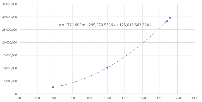
Figure 1. The relationship between water volume and elevation.

The fitting formula has revealed that the primary water supply area of Lake Mead predominantly serves the needs of Las Vegas. To ascertain the annual water requirements, we must calculate the population that necessitates water supply. Given the substantial influx of tourists to Las Vegas, a transient population also factors into this calculation[10]. Therefore, we combine the number of tourists and residents to determine the total water users, represented as

\( \sum n={n_{residents}}+ {n_{tourists}}\ \ \ (12) \)

Using the previously calculated average number of tourists, which amounts to 106,000, we can approximate the annual water demand for tourists as 106,000. Additionally, with the presence of \( 2.699 \) million residents in the area, the total water demand sums up to 2.705 million. Consequently, the approximate value of ‘n’ representing the total water users is \( 2.705 ×{10^{6}} \) .

3.5.5. The definition of a drought. Bring the calculated data into the previous formula to calculate the per year drought water quantity:

\( {V_{supply}} \gt 2 × 3750L × 2.705 × 106 = 16447. 1 acr{e_{feet}}\ \ \ (13) \)

Plot the annual changes of the highest and lowest water levels as follows

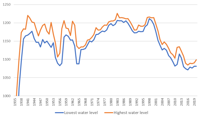
Figure 2. Highest and lowest water level.

Calculate the annual average water level by taking the average of the highest and lowest recorded water levels each year. Then, utilize the fitted relationship between water level and water volume to compute the annual average water volume. Finally, create a graphical representation of the annual average water volume as depicted in the figure below.

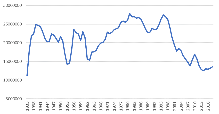
Figure 3. Average water volume.

Calculate \( {V_{supply}} / {V_{average}} \) to determine the proportion of critical water consumption in the total annual water consumption. Compute an average of these ratios as the threshold distinguishing between drought and non-arid conditions. Generate the figure shown below accordingly.

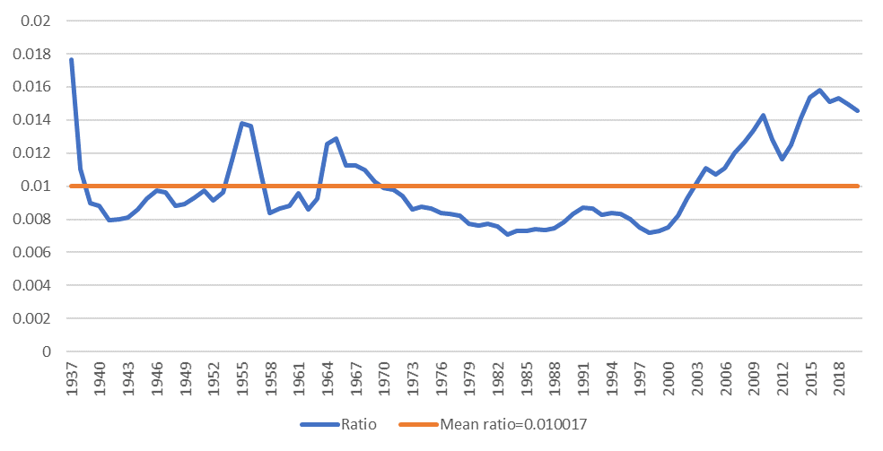
Figure 4. Dry period division.

The standard for defining drought is \( {V_{supply}} / {V_{total}} \gt 0.010017. \) When Lake Mead surpasses this threshold, it is considered to be in a drought state.

According to the drought classification presented in this article, the historical drought periods are as follows:

The first drought period spanned from 1935 to 1938.

The second drought period occurred from 1954 to 1957.

The third drought period extended from 1964 to 1969.

The fourth drought period started in 2003 and ended in 2020

Notably, the second drought period persisted from 2003 to 2020. As depicted in the figure above, it's evident that drought periods are becoming more prolonged, and the severity of drought conditions is increasing.

4. Lake Mead Water Level Forecast

4.1. Model Establishment

This article, based on a review of relevant literature, highlights the intricate interplay of various factors influencing the water levels of Lake Mead. These levels are directly impacted by variables such as rainfall, evaporation, and water consumption. Given the complexity of these dynamic changes, conventional time series forecasting methods prove inadequate.

Therefore, to predict water levels for 2025, 2030, and 2050, this study leverages historical water level data to construct a grey forecast GM (1,1) model. Two distinct datasets, one from a recent drought period and the other spanning from 2005 to 2020, are employed for separate predictions and comparisons.

The grey theory posits that all random quantities can be considered grey quantities, exhibiting variations within defined ranges and timeframes. Instead of seeking statistical laws and probability distributions, data processing aims to convert the original data into regular time series data. Building upon this foundation, mathematical models are established. In this context, the GM (1,1) model based on accumulation is used to generate a sequence of numbers, guided by the following modeling principle.

Step 1: Grade Ratio Test, Modeling Feasibility Analysis

For a given sequence, whether a GM (1, 1) prediction model with higher accuracy can be established, generally the size of the grade ratio and the interval to which it belongs, that is, its coverage, can be judged.

First, we use all the existing values of water level to form a sequence.

\( {x^{(0)}}=({x^{(0)}}(1),{x^{(0)}}(2),{x^{(0)}}(3)......{x^{(0)}}(n)) \) (14)

To get ready to use Grey Model, the grade ratio of the sequence is:

\( {λ^{(0)}}(k)=\frac{{x^{(0)}}(k-1)}{{x^{(0)}}(k)} (here,k=2,3,...,n) \) (15)

For each of the continuous pairs in the sequence, this value should be within the accomodative coverage, for which the formula is

\( λ(k)∈({e^{-\frac{2}{n+1}}},{e^{\frac{2}{n+1}}}) \) (16)

By calculating the grade ratios of the sequence, we can find that all values are within the coverage range. So, the sequence can be modelled by GM (1,1).

Step 2: Data Transformation

The fundamental principle of data transformation processing is ensuring that the level ratio of the processed sequence falls within an acceptable range. This guarantees that for sequences with unsatisfactory level ratios, GM (1, 1) modeling can be carried out following the selected data transformation process. Commonly used data transformations include translation transformation, logarithmic transformation, and square root transformation.

Step 3: GM (1,1) Modeling

Processing the original sequence. Recall the original sequence

\( {x^{(0)}}=({x^{(0)}}(1),{x^{(0)}}(2),{x^{(0)}}(3)……{x^{(0)}}(n))\ \ \ (17) \)

Accumulate it once to get

\( {x^{(1)}}=({x^{(1)}}(1),{x^{(1)}}(2),{x^{(1)}}(3)……{x^{(1)}}(n))\ \ \ (18) \)

where,

\( {x^{(1)}}(k)=\sum _{i=1}^{k}({x^{(0)}}(i))\ \ \ (19) \)

Then, we use the mean value of sequence \( {x^{(1)}} \) to form another sequence.

\( {Z^{(1)}}(k)=\frac{{x^{(1)}}(k)+{x^{(1)}}(k-1)}{2} (here k=2,3,..,63)\ \ \ (20) \)

The cumulative sequence serves to mitigate the volatility and randomness inherent in the original sequence. It transforms the data into a regularly increasing sequence, making it suitable for the development of a predictive model in the form of a differential equation.

Once we have all the required sequences, we can introduce an equation known as the "grey differential equation," expressed as follows.

\( {x^{(0)}}(k)+a{z^{(1)}}(k)=b\ \ \ (21) \)

In the equation, \( a \) and \( b \) are two constants which could be obtained by least square fitting method. First, some martixs should be constructed.

\( u={[a b]^{T}}\ \ \ (22) \)

\( Y={[{x^{(0)}}(2) {x^{(0)}}(3),…{,x^{(0)}}(n)]^{T}}\ \ \ (23) \)

\( B=[ \begin{array}{c} {z^{(1)}}(2) 1 \\ {z^{(1)}}(3) 1 \\ {z^{(1)}}(4) 1 \\ … … \\ {z^{(1)}}(n) 1 \end{array} ]\ \ \ (24) \)

By employing the least square fitting method, the value of " \( u \) " that minimizes the function \( J(u)={(Y-Bu)^{T}}((Y-Bu)) \) is determined as follows:

\( \hat{u}={[\hat{a},\hat{b}]^{T}}={({B^{T}},B)^{-1}}{B^{T}}Y\ \ \ (25) \)

After obtaining values for a and b, the other equation, called “albinism equation”, can be used

\( \frac{d{x^{(1)}}(t)}{dt}+{x^{(1)}}(t)=b\ \ \ (26) \)

Substitute in the above values of a and b and solve the equation, a new sequence \( {\hat{x}^{(1)}} \) could be generated.

\( {\hat{x}^{(1)}}(t)=({x^{(0)}}(1)-\frac{\hat{b}}{\hat{a}}{e^{-\hat{a}k}})+\frac{\hat{b}}{\hat{a}}\ \ \ (27) \)

\( {\hat{x}^{(1)}}(k+1)=({x^{(0)}}(1)-\frac{\hat{b}}{\hat{a}}{e^{-\hat{a}k}})+\frac{\hat{b}}{\hat{a}} (here k=2,3,…,n)\ \ \ (28) \)

Now, to obtain the predicted sequence of the original data, the following transformation is performed based on the previous transformation.

\( {x^{(0)}}(k+1)={x^{(1)}}(k+1)-{x^{(1)}}(k)\ \ \ (29) \)

Step 4: Model Testing

Grade ratio deviation test is used in this model. For a given sequence and its model sequence, the sequence-level ratio and the modellevel ratio are respectively

\( {λ^{(0)}}(k)=\frac{{x^{(0)}}(k-1)}{{x^{(0)}}(k)}\ \ \ (30) \)

\( {λ^{(0)}}(k)=\frac{{x^{(0)}}(k-1)}{{x^{(0)}}(k)}=\frac{1+0.5a}{1-0.5a}\ \ \ (31) \)

Then the level ratio deviation (exponential law difference value) is

\( ρ(k)=\frac{{λ^{(0)}}(k)-{λ^{(0)}}(k-1)}{{λ^{(0)}}(k)}×100\%\ \ \ (32) \)

\( ρ(k)=1-(\frac{1-0.5a}{1+0.5a})\frac{{x^{(0)}}(k-1)}{{x^{(0)}}(k)}×100\%\ \ \ (33) \)

4.2. Model Solving

The simulated values from 2005 to 2020 are:

Table 2. Simulated values from 2005 to 2020.

The forecast value to 2050 is:

Table 3. The forecast value to 2050.

Since the division of the recent drought period in this article is from 2003 to 2020, the forecast result is basically the same as that of 2005 to 2020, so it will not be shown.

The forecast based on 2005-2020 can be clearly shown in the figure below.

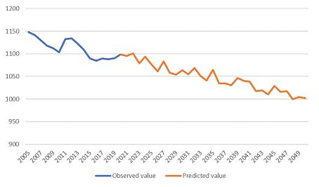
Figure 5. The forecast based on 2005-2020.

5. Wastewater Recycling Program

5.1. Waste Water

5.1.1. Waste Water Source. Urban wastewater comes from three primary sources: domestic, industrial, and rainfall. Domestic: This includes wastewater from daily activities like toilet flushing, bathing, handwashing, and laundry. It originates in homes, schools, public places, and government agencies. It can be divided into domestic sewage (heavily polluted, mainly from toilets) and domestic wastewater (less polluted, from activities like laundry and bathing). Industrial: Compared to industrial wastewater, domestic sewage is easier to recycle. It requires treatment to remove organic matter and meet water quality standards for non-drinking purposes. Wastewater from rainfall, known as stormwater runoff, is difficult to recycle due to its unpredictable and variable composition. It can carry pollutants like debris, chemicals, and sediments from roads and surfaces, making treatment and purification challenging.

5.1.2. Principles of Wastewater Recycling. Sustainability Principle: Treating and reusing urban sewage is crucial for conserving water resources and reducing environmental impact. The process should align with sustainable development principles, focusing on cost-effectiveness and pollution control. Safety Principle: Urban sewage treatment must adhere to national laws and standards while ensuring treated water undergoes rigorous testing. The treated water is suitable for ecological improvements but not for direct human consumption.

5.1.3. Wastewater Recovery Methods. Decentralized Recovery: Small-scale sewage treatment stations in buildings, residential areas, etc., handle sewage generated locally. This method is flexible, cost-effective, and suitable for small areas, reducing pressure on municipal facilities. Centralized Recycling: Large-scale sewage recycling plants collect, treat, and reuse urban domestic sewage. It requires a significant initial investment but offers efficient treatment and wide-scale reuse, contributing to the reliability of the system and sanitary conditions.

5.1.4. Current Wastewater Applications. Urban Landscape Water Bodies: Treated domestic sewage can be used to fill artificial lakes, ponds, fountains, and other landscape features, enhancing aesthetics without compromising water quality. Agricultural Irrigation: Treated sewage can be used for irrigating farmland, conserving drinking-grade water for essential use. Urban Sanitation: Treated sewage finds applications in urban sanitation, such as street cleaning, public green spaces maintenance, and building exterior washing.

5.2. Factors Affecting Wastewater Recovery Plans

Wastewater recovery is influenced by four main factors: financial support, collection pipe network coverage, treatment technology, and wastewater classification capabilities.

Financial Support: Adequate funding is essential for various aspects of sewage treatment and collection, including land purchase, plant construction, equipment maintenance, and pipeline installation.

Collection Pipe Network Coverage: A wider and denser network allows for better utilization of wastewater resources.

Treatment Technology: Effective treatment determines the usability of wastewater. High-quality treatment can lead to drinking-grade water but is costly.

Wastewater Classification Capability: The ability to distinguish wastewater sources enables cost savings and improved water quality through separate treatment.

5.3. Impact Assessment

Assuming that the volume of urban wastewater from the three sources of domestic wastewater, industrial wastewater and rainwater are \( {w_{1}} \) , \( {w_{2}} \) , \( {w_{3}} \) , respectively, their purification rate ratios under certain conditions are \( {f_{1}} \) , \( {f_{2}} \) , \( {f_{3}} \) ,and the purification rate \( {f_{i}} \) is related to the financial support capacity \( {x_{1}} \) , collection of functions related to pipe network coverage \( {x_{2}} \) , treatment technology \( {x_{3}} \) and wastewater classification capacity \( {x_{4}} \) .

\( fi=f(x1, x2, x3, x4)\ \ \ (34) \)

Then the purified water volume \( {W_{0}} \) can be expressed as

\( {W_{0}}=\sum _{1}^{3}{w_{i}}×{f_{i}}\ \ \ (35) \)

The overall purification rate of wastewater \( F \) can be expressed as

\( F=\frac{{W_{0}}}{{W_{1}}+{W_{2}}+{W_{3}}}×100\%\ \ \ (36) \)

6. Conclusion

In Section 3, we examined the factors affecting Lake Mead, including its water levels and drought trends. In Section 4, we created a predictive model for Lake Mead's water levels using historical data. This model allowed us to compare short-term and long-term drought projections. Section 5 focused on key factors in wastewater management, including financial support, collection network size, treatment technology, and wastewater classification.

We aim to consider additional factors affecting Lake Mead's water volume, such as infiltration and plant transpiration. We'll adjust critical water consumption historically based on population data, adopting a dynamic approach. Using monthly water level data, we plan to predict Lake Mead's water levels over the next 30 years. We'll explore training a BP neural network with historical data for more precise predictions.

References

[1]. Robert Jellison, José R. Romero, John M. Melack.The Onset of Meromixis During Restoration of Mono Lake, California: Unintended Consequences of Reducing Water Diversions. LIMNOLOGY AND OCEANOGRAPHY, 1998. (IF: 3)
[2]. Shane A Snyder, Mark J Benotti. Endocrine Disruptors and Pharmaceuticals: Implications For Water Sustainability, 2010. (IF: 3)
[3]. Mark J Benotti, Benjamin D Stanford, Shane A Snyder. Impact of Drought on Wastewater Contaminants in An Urban Water Supply. JOURNAL OF ENVIRONMENTAL QUALITY, 2010. (IF: 3)
[4]. Yu Sun; Susanna T.Y. Tong, Mao Fang; Y. Jeffrey Yang, Exploring The Effects of Population Growth on Future Land Use Change in The Las Vegas Wash Watershed: An Integrated Approach of Geospatial Modeling and Analytics. ENVIRONMENT, DEVELOPMENT AND SUSTAINABILITY,2013. (IF: 3)
[5]. Al Preston, Imad A. Hannoun, E. John List, Ira Rackley, Todd Tietjen. Three-dimensional Management Model for Lake Mead, Nevada, Part 1: Model Calibration and Validation. LAKE AND RESERVOIR MANAGEMENT, 2014. (IF: 3)
[6]. Wei Sun, Xiao Jun Liu. The Prediction for Sewage Emissions in Xi'an Based on The Theory of Grey System. ADVANCED MATERIALS RESEARCH, 2014.
[7]. Xu Wang, Tao Qian, Yanhui Xue; "Water Resource Allocation Based on Optimal Programming", OTHER CONFERENCES, 2022.
[8]. Yixin Li, Predict The Water Level of Lake Mead for The Next 30 Years Based on ARIMA, 2022 INTERNATIONAL CONFERENCE ON FRONTIERS OF ARTIFICIA, 2022.
[9]. C. Deng. Take Lake Mead to Tackle The Drought By Remote Sensing and Two-layer Current Approximation Model. INTERNATIONAL CONFERENCE ON GEOGRAPHIC INFORMATION AND ..., 2023.
[10]. Martha J M Wells; Denise Funk, Gene A Mullins, Katherine Y Bell. Application of A Fluorescence EEM-PARAFAC Model for Direct and Indirect Potable Water Reuse Monitoring: Multi-stage Ozone-biofiltration Without Reverse Osmosis at Gwinnett County, Georgia, USA THE SCIENCE OF THE TOTAL ENVIRONMENT, 2023.
Cite this article
Wu,X. (2023). Prediction of drought in lake mead. Theoretical and Natural Science,13,251-263.
Data availability
The datasets used and/or analyzed during the current study will be available from the authors upon reasonable request.
Disclaimer/Publisher's Note
The statements, opinions and data contained in all publications are solely those of the individual author(s) and contributor(s) and not of EWA Publishing and/or the editor(s). EWA Publishing and/or the editor(s) disclaim responsibility for any injury to people or property resulting from any ideas, methods, instructions or products referred to in the content.
About volume
Volume title: Proceedings of the 3rd International Conference on Computing Innovation and Applied Physics
© 2024 by the author(s). Licensee EWA Publishing, Oxford, UK. This article is an open access article distributed under the terms and
conditions of the Creative Commons Attribution (CC BY) license. Authors who
publish this series agree to the following terms:
1. Authors retain copyright and grant the series right of first publication with the work simultaneously licensed under a Creative Commons
Attribution License that allows others to share the work with an acknowledgment of the work's authorship and initial publication in this
series.
2. Authors are able to enter into separate, additional contractual arrangements for the non-exclusive distribution of the series's published
version of the work (e.g., post it to an institutional repository or publish it in a book), with an acknowledgment of its initial
publication in this series.
3. Authors are permitted and encouraged to post their work online (e.g., in institutional repositories or on their website) prior to and
during the submission process, as it can lead to productive exchanges, as well as earlier and greater citation of published work (See
Open access policy for details).