1. Introduction

In material sciences and engineering, molecular dynamics simulation is one of the technologies that supports us in observing and measuring the structure and dynamics of materials and their properties at a microscopic level [1]. Lennard-Jones potential is widely used for molecular dynamics simulation, and it can describe the potential energy of interactions between atoms and molecules, like Argon [2]. Currently, we have a deep understanding on when and how to employ Lennard-Jones potential to analyze Argon, like calculating the thermodynamic properties and shear viscosity. Most of the simulations ran between Argon atoms (Ar-Ar) or between Argon and Nickel (Ar-Ni). There is no research discussed about the interaction between the mixture of Argon and Argon which have different particle sizes. This article will elaborate in this area. The molecular simulation for the mixture of Argon will be run by Moldy. In Moldy, the distance of two particles when intermolecular potential is zero from Lennard-Jones potential parameters is changed to reach the goal of different sizes of particles. It allows me to observe how the potential energy changes between different sizes of particle. The comparison of the trend of potential energy for different sizes of particles with respect to timesteps is compared by using Gnuplot. It can help us to have a better understanding of the change of potential energy respects to timesteps for different sizes of particles. The purpose of this study is to explore more on potential energy of interaction between molecules under a microscopic level via molecular dynamic aspect.

2. Methodology

Lennard-Jones potential and its relative equation are employed in this article. Lennard-Jones potential is proposed by Sir John Edward Lennard-Jones. It is used to describe the potential energy for the interaction between molecules or atoms based on their separation. The Lennard-Jones potential equation is derived from the difference between attractive forces and repulsive forces. Lennard-Jones potential can be represented by following equation:

\( V(r)=4ε[{(\frac{σ}{r})^{12}}-{(\frac{σ}{r})^{6}}] \) (1)

Or

\( V(r)=\frac{A}{{r^{12}}}-\frac{B}{{r^{6}}} \) (2)

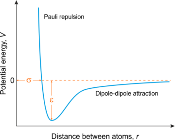
\( V \) is the intermolecular potential energy between two atoms or molecules; \( ε \) is the well depth, which measures how strongly the two atoms attract each other; \( σ \) is the distance between two particles where the intermolecular potential is zero, it is also known as van der Waals radius; \( r \) is the distance between two particles [3]. The Lennard-Jones Potential is usually described as following diagram (Figure 1).

In this article, the simulation is performed by altering the van der Waals radius from the Lennard-Jones Potential equation to change particles’ sizes. The particles’ size is bigger when the van der Waals radius decreases. It means that the particles are closer to each other. The particles’ size is smaller when the van der Waals radius increases. It means that the particles are farther away from each other.

3. Analysis

This section first introduces how the molecular simulation runs based on Moldy and how the data is analyzed using Gnuplot. Then, it discusses the data that is abstracted from Gnuplot and interprets the correlation between the data.

3.1. Framework and background of applied algorithm and technology

In this article, there are two applications that are used, which are Moldy and VMD. Moldy is used to run the molecular-dynamics simulation based on the Lennard-Jones Potential. VMD is used to illustrate the interaction between molecules visually, based on the result from Moldy.

3.1.1. Moldy. Moldy is the C program for running molecular-dynamics simulations of molecules or atoms. The model system contains a mixture of atoms, ions, or molecules in a run-time input file. Rigid-molecule approximation is used to treat molecules or ions, and quaternion methods are used to model their rotational motion. Beeman algorithm is used to present the equations of motion [5]. In this article, the molecular-dynamics simulation runs based on Lennard-Jones Potential for mixtures of Argon. The file for illustrating Argon’s basic information includes Argon’s atomic mass and Lennard-Jones Potential values. The value for the depth of attractive well is 3.984 and interparticle distance is 3.41 for Argon-Argon molecule. There is another file needed to run the simulation for the mixture of Argons. It contains how the simulation performs, like temperature, density, and scale interval.

3.1.2. Gnuplot. Gnuplot is a command-driven program. It can present mathematical functions and data visually [6]. In this article, Gnuplot is used to demonstrate the potential energy for each simulation step for Argon-Argon molecule with different particles’ sizes. It allows us to see the trend of fluctuating potential energy, and the trend for each molecule is compared. In the end, we can have a deep understanding of the molecular interaction between each molecule.

3.2. Data and explanation

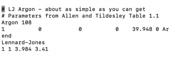
3.2.1. Constant parameters. The constant parameters are the variables that do not change during the simulation. In Moldy, the van der Waals radius ( \( σ \) ) from the file contains basic information that will be changed, and the rest of the information is the same. In Figure 2, 3.41 is the initial value for van der Waals radius, and this value will be modified for further simulation.

Another file contains the code for running simulation for Argon is shown in Figure 3. The information from this file is the same through the entire simulation, which can be defined as independent variables.

3.2.2. Average potential energy respected with variance in van der Waals radius. The van der Waals radius ( \( σ \) ) is changed in this section. The initial value is 3.41 and change the value by increasing or decreasing. The average potential energy is collected. The Table 1 below illustrates how the average potential energy is changed based on the difference in van der Waals radius. The initial value is highlighted in yellow.

Based on Table 1, it is evident to see that the average potential energy increases when van der Waals radius increases, and the average potential energy increases when van der Waals decreases. In other words, the average potential energy is higher when the particles’ size decreases, and the average potential energy is higher when the particles’ size increases. Moldy is unable to process with 5.41 Angstrom for van der Waals radius because the particles are too big, which makes them too close to each other. The graph of average potential energy versus van der Waals radius is portrayed in Figure 4. According to the graph, the change in average potential energy increases slightly when van der Waals radius decreases, and the change in average potential energy increases significantly when van der Waals radius increases from 3.91 to 4.91.

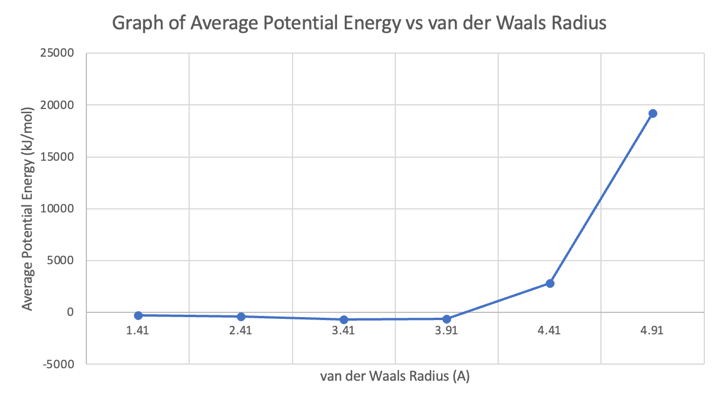
Figure 4. Graph of Average Potential Energy vs van der Waals Radius.

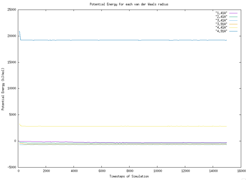
3.2.3. Analysis of trend of potential energy. The potential energy respects to each timestep are depicted graphically by using Gnuplot. The trend for each van der Waals radius is shown in Figure 5. Overall, the trend of potential energy respects to timesteps is similar for the particles with 4.91 Angstrom and 4.41 Angstrom. The trends for the rest are not clear due to large range of potential energy between van der Waals radius of 4.91 Angstrom and 1.41 Angstrom.

The trend comparison for particles with 4.91 Angstrom and 4.41 Angstrom are drawn in Figure 6. From the graph, we know that both start with the highest potential energy, and the potential energy initially decreases until it reaches a point, then the rest seems constant.

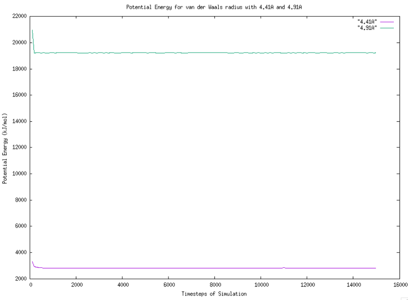
The range of potential energy between van der Waals radius of 4.41 Angstrom and 4.91 Angstrom is large. When both stop decreasing, the trends for potential energy are not very clear and easy to observe. The graph of potential energy with 4.41 Angstrom van der Waals radius is drawn in Figure 7.

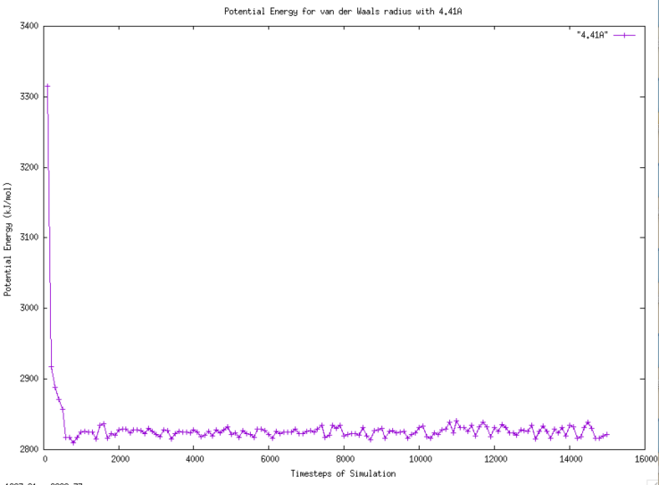
According to Figure 7, it takes approximately 900 timesteps to decrease the potential energy from 3400 kJ/mol to 2830 kJ/mol. The oscillation of potential energy after 900 timesteps follows similar pattern without any outstanding number. The graph of potential energy with 4.91 Angstrom van der Waals radius is drawn in Figure 8.

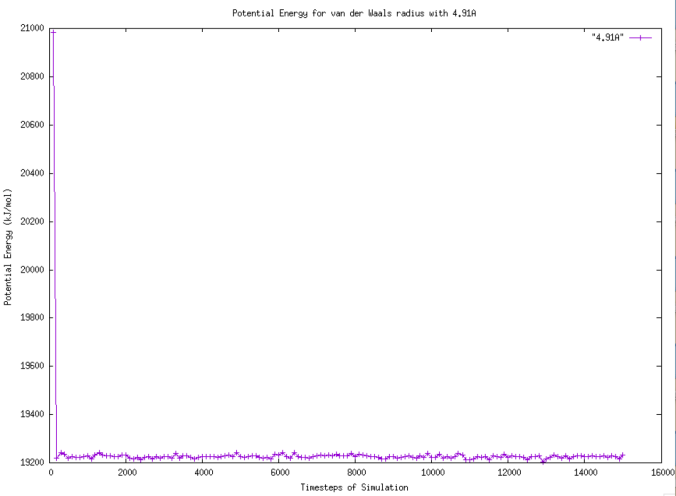
From Figure 8, it is evident to see the potential energy suddenly decreases from the highest potential energy which is about 21000 kJ/mol to approximately 19250 kJ/mol in 100 timesteps. Comparing with Figure 7, the overall trend is similar that the potential energy decreases from the highest potential energy and then the potential energy changes in the similar pattern. The potential energy with 1.41 Angstrom, 2.41 Angstrom, 3.41 Angstrom and 3.91 Angstrom van der Waals radius are compared in Figure 9. To clarify, the data relates to 3.41 Angstrom van der Waals radius is the original one.

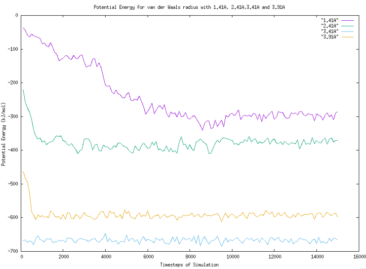
According to Figure 8, there is no sudden change for the molecules with 3.41 Angstrom van der Waals radius. For the molecules with 3.91 Angstrom van der radius, the potential energy decreases significantly in first 300 timesteps from -480 kJ/mol to -600 kJ/mol. Comparing the trend of potential energy with molecules with 4.41 Angstrom and 4.91 Angstrom van der Waals radius, the overall trend is similar which is a sudden decreasing from the highest potential energy to a point where the change of potential energy is insignificant. These three trends have one thing in common that their sizes are all smaller than the original molecules. In addition, we can notice that there is a decreasing for 1.41 Angstrom and 2.41 Angstrom van der Waals radius from the highest potential energy like what happens for particles with 3.91 Angstrom van der Waals radius. However, the decreasing is not sharp. It can be concluded that the change in potential energy at initial timesteps for the molecules that have a bigger size than the original molecule is slow. Vice versa.

4. Conclusion

This article discusses how the potential energy changes with respect to different particle sizes by using Moldy and Gnuplot. Firstly, the article discusses the methodology that is employed, which is Lennard-Jones Potential Function. Then, it introduces the application to run molecular dynamics simulation which is Moldy, and the application to analyze the results from simulations, which is Gnuplot. The analysis is based on Lennard-Jones Potential, and van deer Waals radius is changed to reach the goal. To conclude the result, the average potential energy for each molecule is discovered from Moldy. It is surprising found that the potential energy increases slowly when particles’ sizes increase, and the potential energy decreases significantly when particles’ sizes decrease. The trend of the change of potential energy for each molecule is depicted and compared graphicly from Gnuplot. It discovers that the molecules with changed the sizes have a noticeable change initially, while it does not observe in the original molecule. In addition, the initial decreasing for molecules that increases the size is not as significant as the molecules that decreases the size.

This article has some drawbacks. One drawback is that it does not show visually how the difference in potential energy affects molecules’ movements. In the future, we can try to visualize the molecular movement respect to different potential energy. It can help readers to have a better understanding on molecular interaction for different sizes of particles. Another drawback is that this article does not further discuss why the potential energy increases when particles’ size increases and decreases, and it does not expand on why there is a sudden decreasing for the particles with smaller sizes than origin at initial timesteps. The future can be spent researching those questions.

5. Acknowledgment

I would like to express my special thank for Professor Erik Luijten from Northwestern University. He taught me the knowledge about how to use Moldy to run molecular simulation and how to use Gnuplot to analyze the result from Moldy. He also helped me to target the research topic. In addition, I also want to thank Shuai Yuan who is a graduate student from University of Southern California. He provided a lot of help on coding the Moldy and answered my questions during the simulation. Without their help, this research will not be completed. Finally, I want to thank my parents who offer me this opportunity to study the molecular simulation. It is hard to complete this project without their support.

References

[1]. Landman, U. (1988). Molecular dynamics simulations in material science and condensed matter physics. Springer Proceedings in Physics, 108-123. doi:10.1007/978-3-642-93400-1_12
[2]. Wang, X., Ramírez-Hinestrosa, S., Dobnikar, J., & Frenkel, D. (2020). The Lennard-Jones Potential: When (not) to use it. Physical Chemistry Chemical Physics, 22(19), 10624-10633. doi:10.1039/c9cp05445f
[3]. Libretexts. (2022, August 09). Lennard-Jones potential. Retrieved August 18, 2022, from https://chem.libretexts.org/Bookshelves/Physical_and_Theoretical_Chemistry_Textbook_Maps/Supplemental_Modules_(Physical_and_Theoretical_Chemistry)/Physical_Properties_of_Matter/Atomic_and_Molecular_Properties/Intermolecular_Forces/Specific_Interactions/Lennard-Jones_Potential#:~:text=Proposed%20by%20Sir%20John%20Edward,on%20their%20distance%20of%20separation.
[4]. Generalic, E. (2022, June 29). Croatian-English Chemistry Dictionary & Glossary. Retrieved August 18, 2022, from https://glossary.periodni.com/glossary.php?en=Lennard-Jones%2Bpotential
[5]. Refson, K. (2000). Moldy: A portable molecular dynamics simulation program for serial and Parallel Computers. Computer Physics Communications, 126(3), 310-329. doi:10.1016/s0010-4655(99)00496-8
[6]. Gnuplot homepage. (2022, July). Retrieved August 22, 2022, from http://www.gnuplot.info/
Cite this article
Cheng,Y. (2023). Analyze molecular interaction for mixture of argon and particles with different sizes. Theoretical and Natural Science,18,30-37.
Data availability
The datasets used and/or analyzed during the current study will be available from the authors upon reasonable request.
Disclaimer/Publisher's Note
The statements, opinions and data contained in all publications are solely those of the individual author(s) and contributor(s) and not of EWA Publishing and/or the editor(s). EWA Publishing and/or the editor(s) disclaim responsibility for any injury to people or property resulting from any ideas, methods, instructions or products referred to in the content.
About volume
Volume title: Proceedings of the 2nd International Conference on Computing Innovation and Applied Physics
© 2024 by the author(s). Licensee EWA Publishing, Oxford, UK. This article is an open access article distributed under the terms and
conditions of the Creative Commons Attribution (CC BY) license. Authors who
publish this series agree to the following terms:
1. Authors retain copyright and grant the series right of first publication with the work simultaneously licensed under a Creative Commons
Attribution License that allows others to share the work with an acknowledgment of the work's authorship and initial publication in this
series.
2. Authors are able to enter into separate, additional contractual arrangements for the non-exclusive distribution of the series's published
version of the work (e.g., post it to an institutional repository or publish it in a book), with an acknowledgment of its initial
publication in this series.
3. Authors are permitted and encouraged to post their work online (e.g., in institutional repositories or on their website) prior to and
during the submission process, as it can lead to productive exchanges, as well as earlier and greater citation of published work (See
Open access policy for details).