1. Introduction

Technology in soccer has been booming in recent years. Players’ skills and teams’ tactics are more efficient than they were in the last century, and a lot of new technology has been generated to aid the game. For example, the Video Assistant Referee (VAR) system, introduced to the game in 2018, has profoundly impacted the game’s fairness. “The introduction of VAR has undoubtedly had a significant impact on the game, with decisions now being made with greater accuracy and consistency than ever before” [1]. A decade ago, due to the small-scoring nature of soccer, the only way to get a player’s performance was through statistics, such as the number of goals or assists. But in this case, there was no shortage of players who were nowhere near as good as their stats. Maybe they scored only two goals out of twenty shots, which is a worse performance than a player who scored one goal out of five, but statistically, the former is better. So, “With the emergence of new technologies, soccer clubs can now analyze a vast amount of data to gain insights into player performance, enabling them to make more informed decisions when it comes to player recruitment and team selection” [2].

Expected goals (xG) is a metric used to assess the chance of a shot resulting in a plan which is helpful for coaches and practitioners has been used frequently in recent years to indicate a possible scoring chance on one image and is used in certain other sports (like hockey) [3]. The xG of a shot on goal is usually a number between [0,1], and if a shot on goal is scored, then its xG is 1. A more significant number indicates a higher probability of an attainable goal. Although xG looks like a probability, the media often measures a player’s xG performance over multiple games or a team’s \( xG \) combined, so xG is more like a mathematical expectation. There is no particular uniform definition of xG. While xG may seem like a metric only data analysts care about, xG has emerged and is accepted by the media. Some websites that publish game results and simple statistics often publish xG data for players and teams.”xG has revolutionized the way we analyze soccer matches, providing a more accurate representation of a team’s attacking prowess” [4].

This paper explores the ability of Messi and Ronaldo to score each goal within the sample based on the data required for the xG model to derive the dominance of the two in different situations.

2. Material selection

This paper chose the 2020-2021 season with a similar number of goals scored by both. Messi scored 38 goals, and Ronaldo scored 36. The data was taken from the website “Transfermarkt” and Youtube videos of both players’ plans.

2.1. Data collection

1. Coordinates on the field: “The length of a standard soccer field is 100-110 meters long and 64-75 meters wide. The four corners of the field form a rectangular shape with two goal posts and a crossbar at each end of the field” [5]. We choose the median value of length and width, 105m and 68m. Draw two diagonal lines of the field, with the point of intersection as the origin, as shown in Figure 1. The length is the x-axis, and the width is the y-axis, taking absolute values (no negative numbers). For example, the coordinates of the center point of the goal are (52.5, 0)

2. Shot distance: Meters between the shot location and the central point of the goal line [6]. Using the found x and y coordinates, the straight-line distance between the shot location and the leading end of the goal line is found using the Pythagorean theorem.

3. The shooting area is divided into the customary foot, the non-habitual foot, and other body parts. “The player’s preferred foot is identified as the foot with which they have scored the majority of their goals in the past, while the non-preferred foot is the opposite.” [7]. For example, Messi’s dominant foot is the left foot, while the opposite is true for the non-dominant foot. Other parts of the body are the head or any part of the body other than the foot (hands also count, although they are against the rules, but can be included as long as the referee did not notice and scores, see On June 22, 1986, Maradona handballed the ball into England’s goal during the World Cup quarterfinal match between Argentina and England in Mexico)

4. Visible range of the goal: “The visible range of the goal is defined as the angle between the two goalposts as seen from the ball’s position at the time of the shot.” [8], as shown in Figure 2. It can be found by the law of cosine, which requires knowing the triangle’s three sides. It is known that the goal is 7.3m long, and the line connecting the goalposts can be found using the Pythagorean theorem, and the angle is finally obtained.

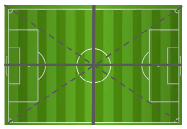
Figure1. Soccer field size.

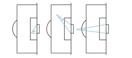
Figure 2. from “Fitting Your Football XG Model · Dato Futbol.”

2.2. Specific data for two players

Table 1 and Table 2, these two tables detail the particular data of Messi and Ronaldo.

Table 1. Messi’s data.

Table 2. Ronaldo’s data.

3. Approach

The datasets, including Time, Visible range of the goal, and Shot Distance, are numerical and can potentially be made into some curve-fitting models. Noticing that the data are dimensional, applying a traditional polynomial regression is impossible. “Probability distribution models are useful tools for modeling soccer data, particularly for analyzing the likelihood of scoring in certain game situations” (Wunderlich, 2019) [9]. So we use a probabilistic model. “Probability distribution models can provide a more accurate and nuanced understanding of soccer data, particularly when dealing with complex, multi-dimensional datasets” [10]. To construct such a model, which can summarize the possibilities of something happening in a particular situation, we decide to split the x-axis intervals into equal-length subintervals and define the density of each subinterval to be the number of goals over the total goals.

So firstly, define

\( [0,{a_{n}}]=[0,{a_{1}})…[{a_{n-1}},{a_{n}}]\ \ \ (1) \)

Denote \( {G_{i}} \) as the goals within each interval; we then have:

\( 1=\sum _{i=1}^{n}\frac{{G_{i}}}{{G_{total}}}\ \ \ (2) \)

The function is then:

\( f(x)=\frac{{G_{i}}}{G}for {a_{i}}≤x≤{a_{i+1}}\ \ \ (3) \)

The area of each “box” is:

\( A={l_{i}}\frac{{G_{i}}}{G} {l_{i}}=length of each interval\ \ \ (4) \)

After constructing the function, we found that the resulting graph is not smooth, contradicting our goals to make a model of comparison. It is continuous, though, so we can still compare through the work by integrating the functions and comparing them with the number. But we still want a visualizable comparison model. The basic idea of density is unchanged, but after researching online, we found a way to smooth the graph -- kernel smoothing.

\( {\hat{f}_{h}}(x)=\frac{1}{nh}\sum _{i=1}^{n}K(\frac{x-{x_{i}}}{h}) \) [11]

Here K() is the kernel smoothing function, n is the sample size, xi is the values of the samples, and h is the bandwidth. The new model is still looking for densities, but it solves the problem of unsmooth by dropping off the term “for.” By assigning weights on different distances though K(), the function enables x to be calculated with the original value of itself. Algebraically the role treats each x as the kernel, which means the distance of the samples to x does not vary from left or right, and the space is the critical part of kernel smoothing. The kernel smoothing function is our desired numeric model, as shown in the figure. Finally, thanks to Matlab, there is a convenience tool called density. The graphs will be made by this tool through Matlab.

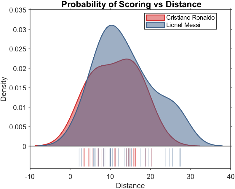
Figure 3. Comparison chart about Shooting Distance.

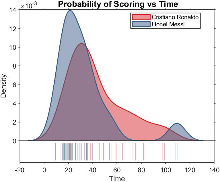
Figure 4. Comparison chart about Game Time.

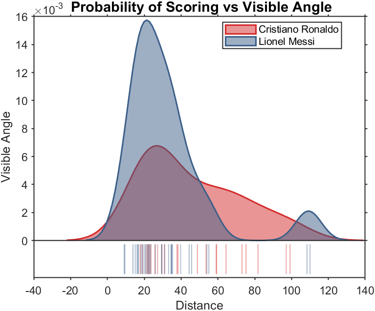
Figure 5. Comparison chart about Shooting visual Angle.

4. Explanation Analysis

Figures 5, 6, and 7 showed several meaningful results. In Figure 5, Lionel Messi shows a distinct advantage compared to Cristiano Ronaldo when the shot is over 20 meters long. In Figure 6, Cristiano Ronaldo shows his strong ability to attack the goal from 60 minutes to 100 minutes of the game. In Figure 7, Cristiano Ronaldo again shows his comprehensive methods to win scores. Also, in the last two figures, we can still see that Lionel Messi is dominantly more decisive than Cristiano Ronaldo when the game comes to his familiar situations. The text only shows the goal preferences of Messi and Crosby in different situations; this model applies to the comparison of any player.

5. Conclusion

In conclusion, this study analyzed the goal-scoring abilities of Lionel Messi and Cristiano Ronaldo based on the 2020-2021 season data and expected goals (xG). Messi demonstrated strength in long-range shots, while Ronaldo displayed versatility in scoring from various situations. The findings provide valuable insights into their respective scoring preferences. This methodology can be extended to compare other players, contributing to player evaluation in soccer. Future research can expand the dataset and employ advanced statistical techniques to enhance the understanding of goal-scoring abilities. Overall, this study contributes to the ongoing debate about Messi and Ronaldo’s scoring abilities and demonstrates the application of numerical models for player comparison in soccer.

References

[1]. Baker, M. (2021). The impact of Video Assistant Referee (VAR) on the fairness of soccer. Journal of Sports Sciences, 39(5), 483-490.
[2]. Kang, S. K., & Lee, S. Y. (2020). The impact of technology on soccer performance analysis. Journal of Physical Education and Sport, 20(1), 95-100.
[3]. Rathke, A. (2017). An examination of expected goals and shot efficiency in soccer. J. Hum. Sport Exer. 12, 514–529. doi: 10.14198/jhse.2017.12. Proc2.05
[4]. Alexander, Duncan. How Soccer Analytics Works. Penguin Random House, 2021.
[5]. Fernández, Javier, and Luke Bornn. “Wide Open Spaces: A Statistical Technique for Measuring Space Creation in Professional Soccer.” Journal of Quantitative Analysis in Sports, vol. 12, no. 3, 2016, pp. 139-150.
[6]. Ismael Gómez, et al. “Fitting Your Own Football XG Model · Dato Futbol.” DATO FUTBOL, 14 Apr. 2020, https://www.datofutbol.cl/xg-model/.
[7]. Lucey, Patrick, et al. “A Multi-Scale Approach to Predicting Goals in Soccer.” Journal of Quantitative Analysis in Sports, vol. 12, no. 4, 2016, pp. 159-168.
[8]. Xu, Qingyang, et al. “Learning to Score in the Wild.” Proceedings of the IEEE Conference on Computer Vision and Pattern Recognition, 2018, pp. 5455-5463.
[9]. Wunderlich, F., & Memmert, D. (2019). Data science and soccer: identifying interesting variables through machine learning techniques. Current Opinion in Psychology, 34, 155-159.
[10]. Bialkowski, A., Lucey, P., Carr, P., & Matthews, I. (2014). Probabilistic event forecasting in soccer. In Proceedings of the 23rd international conference on World Wide Web (pp. 557-562). https://www.mathworks.com/help/stats/ksdensity.html
Cite this article
Chen,X.;Tang,Y. (2023). Judging Messi’s and Ronaldo’s scoring ability in different situations according to the model. Theoretical and Natural Science,28,123-128.
Data availability
The datasets used and/or analyzed during the current study will be available from the authors upon reasonable request.
Disclaimer/Publisher's Note
The statements, opinions and data contained in all publications are solely those of the individual author(s) and contributor(s) and not of EWA Publishing and/or the editor(s). EWA Publishing and/or the editor(s) disclaim responsibility for any injury to people or property resulting from any ideas, methods, instructions or products referred to in the content.
About volume
Volume title: Proceedings of the 2023 International Conference on Mathematical Physics and Computational Simulation
© 2024 by the author(s). Licensee EWA Publishing, Oxford, UK. This article is an open access article distributed under the terms and
conditions of the Creative Commons Attribution (CC BY) license. Authors who
publish this series agree to the following terms:
1. Authors retain copyright and grant the series right of first publication with the work simultaneously licensed under a Creative Commons
Attribution License that allows others to share the work with an acknowledgment of the work's authorship and initial publication in this
series.
2. Authors are able to enter into separate, additional contractual arrangements for the non-exclusive distribution of the series's published
version of the work (e.g., post it to an institutional repository or publish it in a book), with an acknowledgment of its initial
publication in this series.
3. Authors are permitted and encouraged to post their work online (e.g., in institutional repositories or on their website) prior to and
during the submission process, as it can lead to productive exchanges, as well as earlier and greater citation of published work (See
Open access policy for details).