1. Introduction

Unemployment rate is an important economic indicator reflecting the utilization of labour resources in a country or region, and it is the main goal of adjusting macroeconomic policies in various countries. Generally speaking, the rising unemployment rate means that more labor force cannot be fully utilized. With the increase of unemployment, the total demand of society will gradually decline, and the driving force of economic growth will be weakened. Therefore, governments use the unemployment rate as an important basis for judging the degree of economic health when adjusting domestic economic and monetary policies and supply and demand relations [1].

Time series analysis is a statistical method used to analyze and predict time series data [2]. Its goal is to understand the patterns, trends and periodicity in the data, and to predict and make decisions accordingly. The researches have a wide range of applications in many fields, including medicine [3, 4], economics [5], finance [6], meteorology [7]. According to the monthly data of the U.S. unemployment rate (USUR) from the U.S. Bureau of Labor Statistics [8], the proportion of total employment in the United States is gradually increasing, but the unemployment rate fluctuates greatly. Among them, the period in which the unemployment rate in the United States grew more rapidly is roughly 1975-1977, 1980-1986 and 2008-2009, which correspond to the United States inflation, the oil crisis and the global financial crisis. The research of Xue [9] and Shao [10] shown that the monthly data of unemployment rate in the United States can be analyzed by time series analysis method to fit the model and predict the unemployment rate in the future.

By observing the monthly data of the unemployment rate in the America since January 1948, researches established an ARIMA model for USUR for fitting, analysis and prediction [11]. The lack of literature can be attributed to the following points: Take the industrial structure, national macroeconomic regulation and monetary policy as the starting point for analysis and research. Most of the domestic data are used as research samples, and there is no comparative analysis of other countries. The object of analysis is limited to the urban or overall unemployment rate, and there is a lack of analysis of the employment of young people [12]. The establishment of the model only uses the unemployment rate of the United States, and analyzes it against the background of the US market economic system. There is no expansion of the scope to establish a more universal time series prediction model, and there is a lack of a control group under similar economic systems.

In this paper, the influence of the stability and seasonality of time series on the model is considered when establishing the model. In order to increase the stationarity of the data to correctly establish the model, logarithmic preprocessing, residual white noise test and differential unit root test are used. Considering the influence of seasonality, after consulting the data, we choose to add seasonal factors to the original ARIMA model. After comprehensive consideration and comparison, we choose a more appropriate prediction model to predict the unemployment rate of the United States in the next 24 periods.

2. Methods

2.1. Data source

The U.S. data used in this paper is derived from the official database of Labor Statistics, and selects the monthly unemployment rate data of the United States from January 1948 to January 2019. Firstly, the time series diagram of the data is drawn, such as Figure 1.

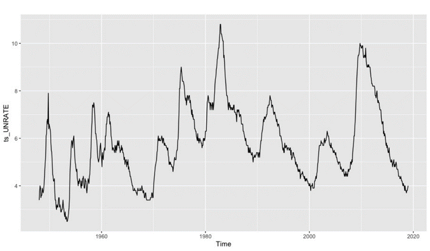
Figure 1. Unemployment Rate of China and US.

In Figure 1, we can find that the unemployment rate in the U.S. is up to its lowest in 1954 and reached its highest in 1984. From 2008 to 2009, due to the impact of the global economic crisis, the U.S. unemployment rate grew rapidly. It can be seen from the time series diagram that the fluctuation of unemployment rate in the United States is regular, so the unemployment rate in the U.S. may have seasonal factors.

In addition, seeing the large time span of the selected data and the large fluctuation of the unemployment rate data, the logarithm of the time series data is stable.

2.2. Model selection

The main purpose of analysis of time series is to predict future nodes based on the data corresponding to historical time. The commonly used prediction models are AR model, MA model, ARMA model, ARIMA model and SARIMA model. Among them, the ARIMA model has been applied by many scholars in different fields to analyze and predict time series. According to the time series image of the selected data, it is speculated that the selected data may be seasonal. This paper will use ARIMA to analyze the time series of the unemployment rate in the United States, and add seasonal factors to the model. This paper selects the unemployment rate from January 1948 to December 2016 as the sample set to determine the parameters of the model for fitting, and then uses the unemployment rate data from January 2017 to January 2019 as the test set to substitute into the model for prediction.

3. Results and discussion

3.1. ARIMA model

The standard form of ARIMA model is ARIMA(p, d, q), where AR and MA represent autoregressive process and moving average process respectively. The parameters p and q are the autocorrelation order and the moving average order. Parameter d represents the difference order required to convert a non-stationary sequence into a stationary time series. In the data preprocessing part, in order to make the unemployment rate more stable, the logarithm is taken. However, according to the autocorrelation test, as shown in Figure 2, we find that the autocorrelation is strong and the ACF function continues to tail, so the time series data is still non-stationary.

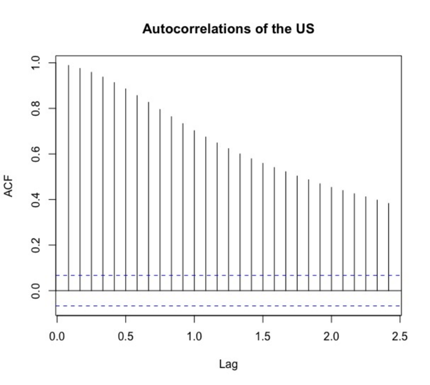
Figure 2. Autocorrelations of the US.

The time series data after logarithm is still not stable, so in order to make the time series more stable and facilitate the establishment of the model, we perform first-order difference and second-order difference on the training sample data after logarithm. According to the improved unit root test (ADF test) based on the Dickey-Fuller test, the p values of the first-order difference and the second-order difference are both less than 0.01, so the null hypothesis (the time series is unstable) is rejected on the basis of the 99 % confidence interval, that is, the first-order difference and the second-order difference are both stationary time series. As hinted in Table 1.

Table 1. ADF test of the first-order-difference and the second-order-difference.

It can be told from Figure 3 and Figure 4 that the 2nd-difference is more stable than the first harmonic coil order difference. In terms of volatility, the fluctuation degree of the 1st-difference is greater than that of the second-order difference. The data after the first difference is between 0 and 0.05, while that after the second difference is between 0 and 0.03. Therefore, the parameter d is 2. Therefore, the model can be set to ARIMA (p, 2, q). Next, we do the ACF graph (Figure 5) and the PACF graph (Figure 6) of the second difference. From the graph, we can see that the autocorrelation function is second-order truncated, so q can be taken as 0,1,2, and the partial autocorrelation coefficient is fourth-order truncated, so 0,1,2,3,4 can be taken.

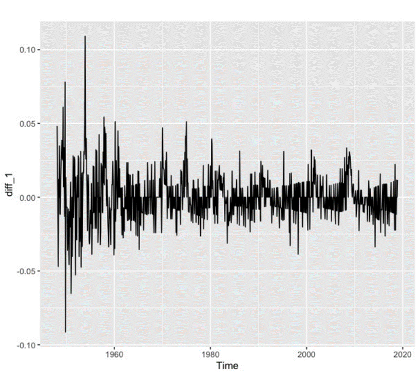
Figure 3. Autocorrelations of the US.

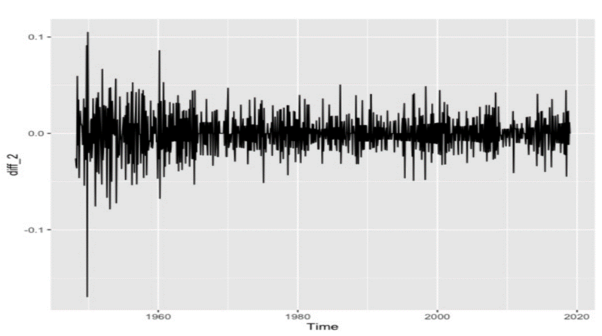
Figure 4. The second-order-difference.

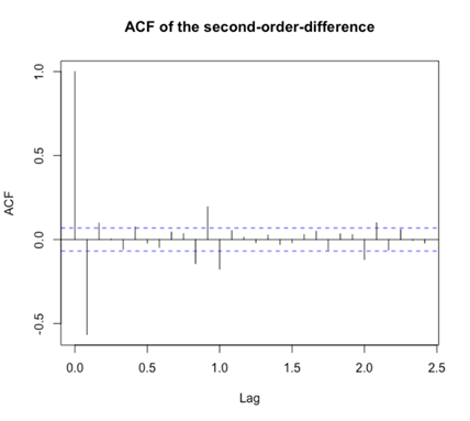
Figure 5. ACF of the second-order-difference.

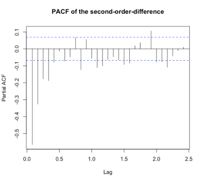
Figure 6. PACF of the second-order-difference.

From the above analysis, 15 possible ARIMA models can be obtained. In order to select the most suitable parameter values, the MSE, AIC and BIC of different parameter values in the ARIMA model are compared. The training set is used to test the regression prediction results of 15 models. The lower values of MSE, AIC and BIC are, the more suitable the fitting degree of the model is. Table 2 shows the results of the 15 models.

Table 2. ARIMA model results

From Table 2, it is found that the minimal values of MSE, AIC and BIC are appeared in the model of ARIMA (2,2,4), which is the best fit among all 15 models. Combining the predicted value of ARIMA (2,2,4) with the actual image of the training set, as shown in Figure 7. It can be found that the fitting effect of the predicted value of the model fitting and the original real data is not good, indicating that seasonality has a great influence on the fitting prediction effect of the ARIMA model.

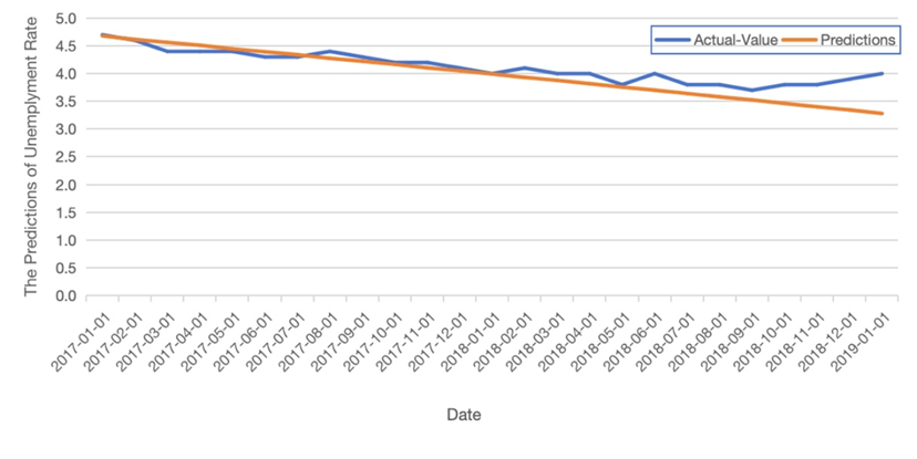
Figure 7. Plot of the predict value.

3.2. SARIMA model results

SARIMA is seasonal ARIMA, which can be expressed as SARIMA (p, d, q) × (P, D, Q) [S]. The first half represents the non-seasonal part, and the second half denotes by the seasonal part, where S represents the seasonal frequency. The auto.arima function can be used to automatically determine the order in R, and the AICc criterion is the default criterion. The results are shown in Table 3.

Table 3. Coefficients of the ARIMA(3,1,1)(2,0,2)[12]

From the running results, it can be concluded that the model SARIMA(3,1,1) ×(2,0,2)[12] fits best as to the value of AIC=-384.13,AICc=-383.9 and BIC = -341.79. Therefore, we use the results of this model to fit the training set and predict the time series of the test set. The fitting error RMSE = 0.1886159 < 0.5 of the training set can be obtained (table 4).

Table 4. Results of error measures

The model’s residuals are calculated and the Box-Ljung Test is used to determine whether the residuals are significant, so as to test whether the residuals are white noise sequences. The running results are shown in Table 5, p-value = 0.9606 > 0.05, indicating that the residual sequence accepts the null hypothesis under the 95 % confidence interval and is already white noise. There is no autocorrelation in the time series data, and the model fully extracts the effective information in the data (Figure 8).

Table 5. The results of Box-Ljung test

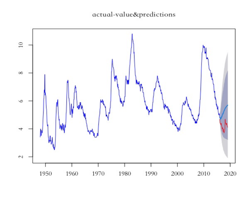
Figure 8. Prediction and actual values’ comparison.

4. Conclusion

In this paper, ARIMA(2,2,4)and SARIMA(3,1,1)×(2,0,2)[12]are used to fit the time series of the US unemployment rate. In the fitting process, this paper finds that the RMSE of ARIMA(2,2,4)is 0.2023, while the RMSE of SARIMA(3,1,1)×(2,0,2)[12] is 0.1886159, which is slightly lower than that of ARIMA(2,2,4). Therefore, the optimal model for fitting the time series data of USUR from January 1948 to December 2016 is SARIMA(3,1,1)×(2,0,2)[12], so SARIMA(3,1,1)×(2,0,2)[12] can better predict the change of USUR from January 2017 to January 2019. However, from the experimental results of this paper, the final prediction effect of the two models is not very good, and there may be other macro variables that this paper ignores that have a certain impact on the change of time series data. In the future, more in-depth exploration can be carried out to find other influencing factors and more optimized fitting prediction schemes.

References

[1]. Cai F 2019 Giving priority to employment at the macro policy level is suitable for the needs of China ‘s current employment situation, and the corresponding concept transformation and mechanism adjustment are at the right time. Financial circles, 13, 37-40.
[2]. Yang S F 2015 Time series modeling and prediction. Tsinghua University.
[3]. Peng Z X, et al. 2008 ARIMA multiplicative seasonal model and its application in the prediction of infectious diseases. Mathematical statistics and management, 2, 362-368.
[4]. Ren Z H 2013 Temporal epidemiological characteristics and trends of pulmonary tuberculosis in China from 2005 to 2011. China Health Statistics, 30 (02), 158-161.
[5]. Li J 2022 Research on the economic growth prediction model of China ‘s tertiary industry based on time series analysis. Suzhou University of Science and Technology.
[6]. Tao Z F, Feng H Y and Chen H Y 2023 IO-type outlier detection method for interval-valued time series and its application in financial time series analysis. Operation Research and Management, 32 (04), 118-125.
[7]. Xue L R 2013 Analysis of the U.S.unemployment rate based on time series. China Foreign Investment, 6, 242-245.
[8]. Shaopeng C 2020 Research on US unemployment rate prediction based on ARIMA time series model. International Public Relations, 12, 395-396.
[9]. Liao M Q 2022 On the practical application of ARIMA mathematical model. China Association for the Advancement of International Science and Technology International Academician Consortium Working Committee.
[10]. Shen X D 2019 A review of time series algorithms based on deep learning. Information technology and informatization, 1, 71-76.
[11]. Liu N and Liu C 2014 An Analysis of the Impact of Delayed Retirement on Young People ‘s Employment - Based on Data from 29 Provinces and 18 Industries in China. Southern Population, 29 (02), 27-35.
[12]. Zhang W, Zhang Y Q and Yang X 2002 Time series data ARIMA seasonal product model and its application. Journal of the Third Military Medical University, 8, 955-957.
Cite this article
Zou,X. (2024). U.S. unemployment rate prediction using time series model. Theoretical and Natural Science,30,255-262.
Data availability
The datasets used and/or analyzed during the current study will be available from the authors upon reasonable request.
Disclaimer/Publisher's Note
The statements, opinions and data contained in all publications are solely those of the individual author(s) and contributor(s) and not of EWA Publishing and/or the editor(s). EWA Publishing and/or the editor(s) disclaim responsibility for any injury to people or property resulting from any ideas, methods, instructions or products referred to in the content.
About volume
Volume title: Proceedings of the 3rd International Conference on Computing Innovation and Applied Physics
© 2024 by the author(s). Licensee EWA Publishing, Oxford, UK. This article is an open access article distributed under the terms and
conditions of the Creative Commons Attribution (CC BY) license. Authors who
publish this series agree to the following terms:
1. Authors retain copyright and grant the series right of first publication with the work simultaneously licensed under a Creative Commons
Attribution License that allows others to share the work with an acknowledgment of the work's authorship and initial publication in this
series.
2. Authors are able to enter into separate, additional contractual arrangements for the non-exclusive distribution of the series's published
version of the work (e.g., post it to an institutional repository or publish it in a book), with an acknowledgment of its initial
publication in this series.
3. Authors are permitted and encouraged to post their work online (e.g., in institutional repositories or on their website) prior to and
during the submission process, as it can lead to productive exchanges, as well as earlier and greater citation of published work (See
Open access policy for details).