1. Introduction

The U.S. real estate market has long been the cornerstone of the U.S. economy, with housing prices being a key indicator of economic health and stability. Since 1991, U.S. real estate prices have gone through several cyclical fluctuations. Significantly, the collapse of the real estate bubble in 2007 triggered a substantial drop in housing prices, profoundly affecting the U.S. economy [1]. Moreover, there was a close relationship between the House Price Index (HPI) and gross domestic product (GDP) before, during, and after the 2007-2008 mortgage and financial crisis [2]. However, the COVID-19 pandemic has caused unprecedented disruption to the real estate market; it has made people more inclined to live in non-central urban areas with lower population density and warmer climates [3]. Lockdowns, shifts to remote work, and changes in consumer preferences have led to a surge in housing demand, pushing housing prices in many areas to record highs. According to Redfin, the median U.S. home price in June 2024 was $442,451, up 4% from the previous year [4]. The sudden surge in housing prices has raised concerns about affordability and sustainability, and accurate forecasts are more important than ever. Therefore, there are many factors that affect housing prices, covering all aspects. Examining past trends and forecasting future factors that influence the real estate market and housing prices, along with understanding their significance, can enable individuals to make informed decisions in investment, financial planning, or home purchases. This, in turn, supports the healthy and stable growth of the real estate market.

However, the real estate market encountered unprecedented challenges as a result of the COVID-19 pandemic [5]. Severe infections have led people to prefer living in less densely populated, warmer, non-central urban areas; many people have moved from New York City to the Northeast and West of the United States [3]. Boston's real estate market was also affected by the epidemic, but it still maintained a relatively high level of housing prices. Boston, being one of the United States' most historic cities, boasts abundant educational resources and robust economic sectors like healthcare and technology, which have bolstered the city's stable job market and, in turn, increased the demand for housing. Therefore, high demand has kept Boston's housing prices at a high level during the epidemic.

Scholars have proposed a variety of methods to predict housing prices, such as the Markov prediction model [6]. This paper will use the random forest algorithm to predict housing prices. This algorithm is highly praised for its excellent performance and wide application. The random forest algorithm can handle various types of data patterns and is particularly good at capturing complex underlying trends and seasonal changes, which are particularly important in housing price prediction. Housing prices in the real estate market are influenced by various complex factors, such as economic conditions, policy shifts, and seasonal changes. By incorporating these multidimensional factors, the random forest algorithm can yield more accurate and stable predictions [7]. As a result, this paper selects the random forest algorithm to address the challenges of predicting housing prices and aims to achieve reliable outcomes in a complex market environment.

2. Methodology

2.1. Data Sources

Choosing a suitable dataset is the key to the success of a machine learning project [8]. An ideal dataset not only needs to provide enough information to support model training but also must be diverse and extensive to ensure good generalization of the model. The Boston House Price Dataset is popular for its completeness, clear variable definition, and good representativeness, and is therefore often used in various house price prediction studies.

As a long-standing dataset, the Boston House Price Dataset has been widely studied, and its related literature and research results have high reference value [9, 10]. The dataset covers a variety of features closely related to house prices, such as crime rate, number of rooms, tax rate, etc., which are all important variables affecting house prices. Due to the moderate size of the dataset (containing 506 data points), it is very suitable for training and testing machine learning models, allowing researchers to obtain effective prediction results at a reasonable computational cost.

2.2. Feature explanation

Table 1 shows 13 feature information and 1 price information in the Boston House Price Dataset. The first column lists the abbreviations of the features, and the second column provides detailed explanations of these features. These features are important reference factors affecting house prices.

Table 1. Characteristics of Boston housing price dataset

2.3. Variable selection

In machine learning, especially regression problems, commonly used indicators for evaluating model performance include R-squared ( \( {R^{2}} \) ), Mean Absolute Error (MAE), Mean Squared Error (MSE), and Root Mean Squared Error (RMSE) [11]. These evaluation metrics offer various insights into the model's performance in predicting housing prices. \( {R^{2}} \) reveals the explanatory power of the model; MAE and RMSE provide the absolute size of the error; and MSE emphasizes the penalty for large errors. By integrating these metrics, the model’s performance can be thoroughly assessed, ensuring it captures overall housing price trends while minimizing errors in specific predictions [12].

2.4. Model selection

By integrating the outputs of numerous decision trees, Random Forest serves as an ensemble learning method that boosts prediction accuracy. It is an improved combination algorithm based on classification trees based on the bagging algorithm. The algorithm is composed of many unpruned decision trees. The core concept involves applying the bootstrap resampling method to randomly select k sample sets, with replacement, from the original dataset to create new training sets. These k new training sets are then used to generate k decision trees, which together form a random forest for classifying or regressing the test set data [13].

During the model training process, each decision tree is trained based on randomly selected samples and features [14]. Since the training samples and features of each decision tree are different, the generated trees are diverse. In classification tasks, Random Forests reach the final decision through a majority vote, while in regression tasks, they produce the final prediction by averaging the outputs of all the individual trees.

Random forest is implemented based on the bagging theory. Random forest uses a decision tree as the base classifier model after bagging [15]. First, the original data set is randomly sampled using the Bootstrap method to generate multiple training sets and corresponding test sets. A decision tree is trained for each training set. The decision trees under different training sets are independent of each other. These decision trees constitute a random forest. Moreover, when building a decision tree, a random subset of features is selected from the complete set of attributes in the training data. This subset serves as the split criteria for the current node of the tree. Throughout the creation of the random forest model, the size of this random feature subspace remains consistent. These are also the two most critical random steps in a random forest. Finally, the classification result is generated by voting on each decision tree. Since the bagging algorithm used by random forest is an integrated learning algorithm, both samples and features are randomly sampled, thus avoiding overfitting. The bagging process is shown in Figure 1.

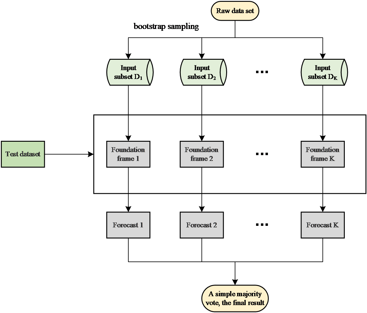
Figure 1. Bagging process diagram

The random forest algorithm follows these steps:

Step 1: The Bagging algorithm is applied to randomly draw k sample sets from the original dataset S, forming new sub-training sets. These k sample sets are then used to build k CART decision trees.

Step 2: During the training phase of each CART regression tree, when the dataset contains M features, the algorithm randomly selects m features (where m < M) for each node. From the chosen features, the algorithm determines the optimal split point to separate the data into left and right subtrees, repeating this process until a predetermined stopping criterion is reached.

Step 3: Following the process in Step 2, k CART regression tree models are constructed.

Step 4: The final prediction for each CART regression tree is determined by calculating the mean of the leaf nodes corresponding to the sample point.

Step 5: The random forest's final prediction is achieved by averaging the outputs from all k CART regression trees.

Figure 2 describes the generation process of the random forest.

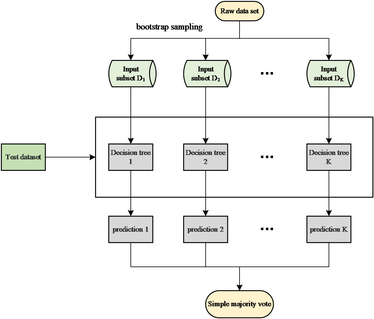
Figure 2. Generation Process Diagram of random forest

3. Results and discussion

3.1. Data visualization analysis

The random forest model is not like some algorithms that require data normalization (such as SVM or K nearest neighbor). Decision trees are essentially based on rule-based partitioning of space, so the scale of the data does not have to be consistent. In the Boston housing price data set, the data distribution is shown in Figure 3, with the characteristics of right-skewed distribution, outliers, and multi-peak distribution. The robustness of the random forest model and its ability to handle nonlinear relationships can effectively deal with the characteristics existing in the data. This paper directly inputs these features into the random forest model without doing too much data preprocessing.

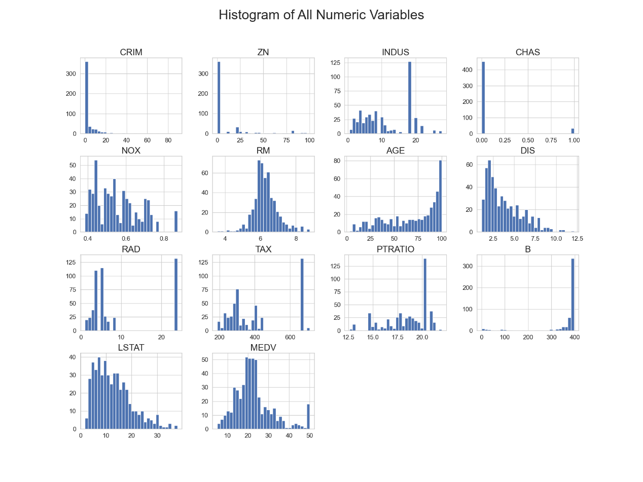
Figure 3. Boston housing price dataset feature data distribution

3.2. Random forest Model Prediction

Figure 4 and 5 present a direct comparison between the actual values and the predicted values when the Random Forest model was trained and tested on the Boston housing price dataset. Table 2 provides the evaluation metric values for the Random Forest model during both the training and testing phases. The R^2 value on the training set is close to 1, indicating that the model can fit the training data well. It is also reflected in the scatter plot of Figu 4 of the training set. The scatter points of the actual value and the predicted value are basically distributed near the diagonal, indicating that the model almost perfectly predicts the training data. The \( {R^{2}} \) value on the test set is 0.8875. Although it has decreased compared with the training set, it still shows good predictive ability. Figure 5's scatter plot of the test set reveals that while most predicted values closely align with actual values, there is a slight bias in the predictions for some extreme values, particularly in the higher housing price range where the model's accuracy diminishes. Nevertheless, the random forest model overall demonstrates strong performance. This is due to the adaptability of the random forest model to multiple feature types. The random forest can flexibly respond to these features by integrating multiple decision trees and making full use of this feature information to improve the prediction performance. Additionally, the Random Forest model enhances its generalization ability and mitigates overfitting by incorporating randomness, such as through the random selection of features and samples during the construction of each tree.

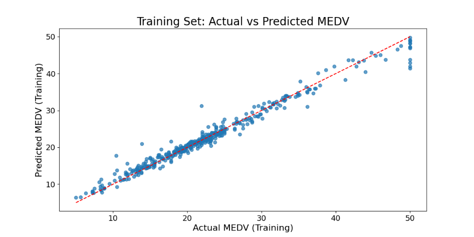
Figure 4. True value and predicted value during random forest model training

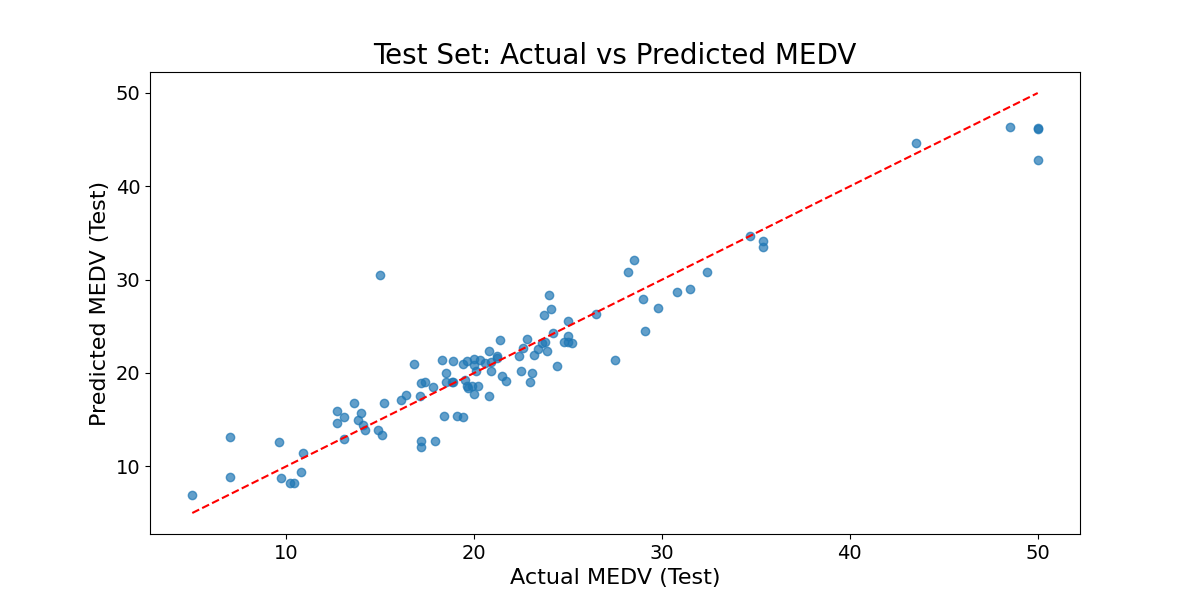
Figure 5. True value and predicted value when testing the random forest model

Table 2. Random forest Model Performance

3.3. Comparison results of various methods

To evaluate the performance of the Random Forest model on a specific dataset, this paper compared it with three other models: Multiple Linear Regression, XGBoost, and Support Vector Machine (SVM) [16-18]. Multiple Linear Regression is a conventional approach that fits a linear equation to multiple features to minimize the difference between predicted and actual values. XGBoost, or Extreme Gradient Boosting, is an ensemble technique that improves prediction accuracy by combining several weak classifiers, usually decision trees, and assigning different weights to each. The Support Vector Machine is a supervised learning model used widely for classification and regression, which distinguishes classes or predicts continuous values by finding the optimal hyperplane in a high-dimensional space.

Table 3 shows the performance comparison of the four models. It can be clearly seen that random forest outperforms other models in all evaluation indicators. The mean square error (MSE) and root mean square error (RMSE) of multiple linear regression and support vector machine are higher, and the coefficient of determination ( \( {R^{2}} \) ) is lower, indicating that they are obviously insufficient in capturing the complexity and nonlinear relationship of data. Although XGBoost performs better than multiple linear regression and support vector machines, its error is still higher than random forest and its \( {R^{2}} \) is slightly lower.

Multiple linear regression and support vector machines are primarily good at capturing linear relationships and therefore perform poorly when faced with the complex nonlinear relationships that may exist in the Boston housing price data set. In contrast, Random Forest and XGBoost, as ensemble learning methods, significantly improve prediction performance by combining multiple weak models. Random forest constructs multiple decision trees by randomly selecting features and samples, which effectively reduces the bias and variance of a single model. XGBoost optimizes the model through gradient boosting trees, but due to its complexity and the need for parameter tuning, its performance on some data sets may be slightly worse than random forest.

Random forests are particularly good at dealing with noise and outliers because they integrate the predictions of multiple decision trees, reducing the sensitivity of a single decision tree to noise. As a result, random forests excel in dealing with complex data and reducing model bias, outperforming multiple linear regression, support vector machines, and XGBoost. Its integrated learning method and noise resistance give it higher accuracy and stability in practical applications.

Table 3. Performance comparison of various methods

To clearly illustrate the benefits of the random forest model compared to other models, this article uses three distinct colors in the comparison chart to represent the predicted and actual values. Green circles represent sample points where all models perform well, red crosses represent sample points where all models perform poorly, and blue boxes represent sample points where the random forest model performs well but other models perform poorly.

When marking these sample points, this paper used different error thresholds. The green threshold is set to the 25th percentile of the error distribution, indicating sample points with small errors and that all models can fit well. These points usually have typical characteristics and obvious patterns. The red threshold is set to the 60th percentile of the error distribution, indicating sample points that are difficult for all models to fit. These points may contain outliers, noise, or complex features, resulting in large prediction errors. The blue threshold is set to the 60th percentile of the random forest model error distribution to mark sample points where random forests perform well but other models perform poorly. These points usually contain complex nonlinear relationships or outliers. Random forests, due to their advantages in ensemble learning, can better capture these complex patterns and thus perform well at these points.

Through these marks, the performance of each model in different situations is obvious. For example, the sample points marked with green circles have smaller errors, indicating that the characteristics of these sample points are more typical and all models can accurately predict. The sample points marked with red crosses have larger errors, which may be due to outliers or complex features, making it difficult for all models to accurately predict. The sample points marked with blue boxes are areas of special concern, showing that random forests can still maintain good prediction performance in complex situations that other models have difficulty dealing with, which shows that random forests have strong nonlinear processing capabilities and robustness. Even for the challenging sample points marked with red crosses, the random forest model outperforms the other models, further emphasizing its effectiveness in managing noise and outliers (Figure 6).

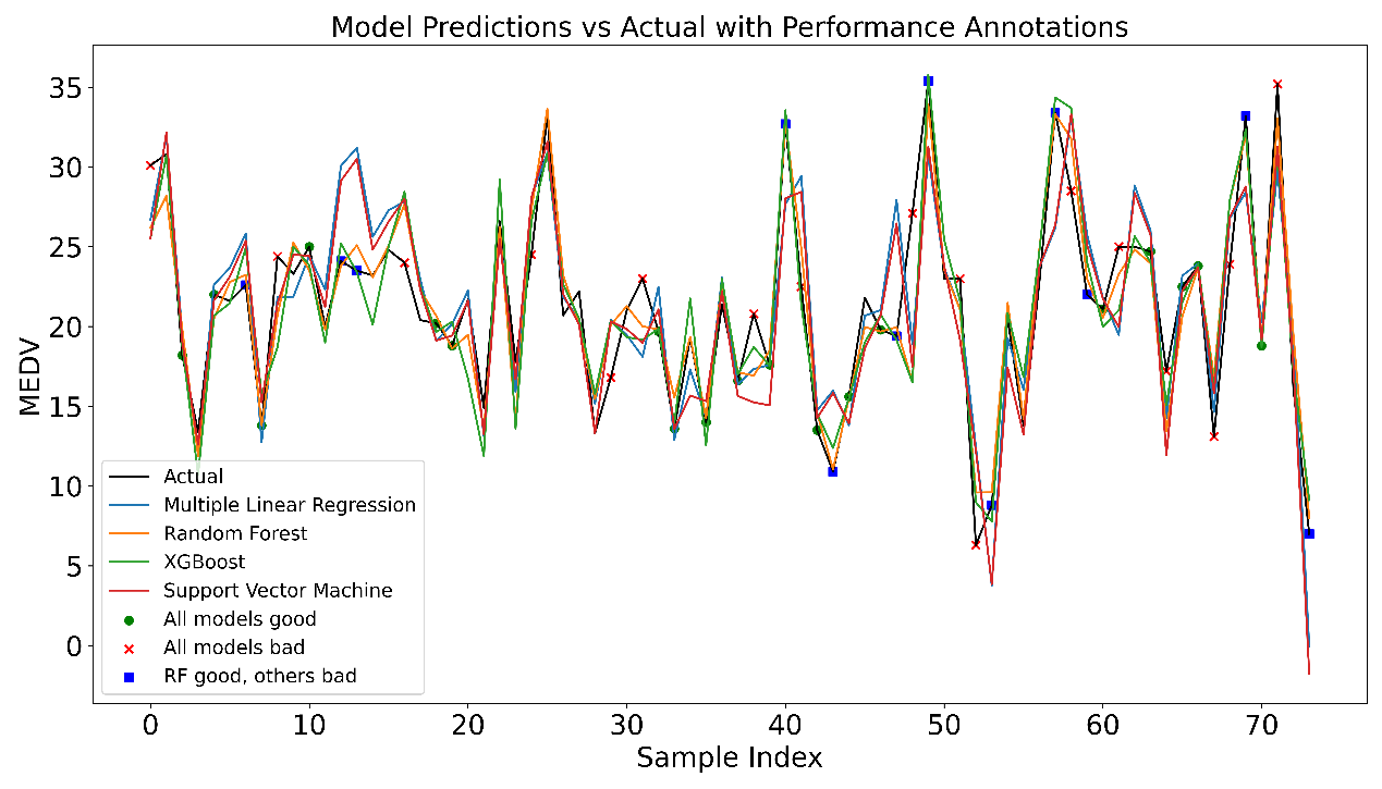
Figure 6. Comparison of prediction performance of different models

3.4. Feature Impact

The Boston housing price dataset contains 13 features and 1 median housing price. To identify which features most significantly affect prices and which feature variations have the most noticeable impact, the feature importance scores from the random forest model can be analyzed [19].

The feature importance score is used to assess how much each feature contributes to the model's predictions. In the Random Forest model, this score is determined by evaluating the feature's influence in the tree-splitting process [20]. Specifically, the model tracks the information gain (such as the reduction in impurity) achieved by each node split and then computes the average information gain a feature contributes across all decision trees to derive its importance score. Common impurity measures used in this context include Gini impurity and information gain.

Table 4. Features and feature importance

The feature importance score chart is shown in Figure 7, and the detailed values of the feature importance score are shown in Table 4. Number of rooms has the highest importance score at 0.55. This shows that the number of rooms has the greatest impact on house prices. Typically, an increase in the number of rooms means a larger house, greater comfort, and therefore higher housing prices. This is followed by the low-income population ratio, whose importance score is approximately 0.32. This shows that the proportion of low-income people has a significant impact on housing prices. Areas with a higher proportion of low-income people generally have lower housing prices, and vice versa.

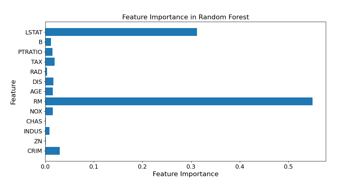
Figure 7. Feature importance score

Other features such as crime rate, air pollution index, house age, and distance to the city center have lower importance scores, with scores of each feature ranging from approximately 0.02 to 0.05. Although these features have some impact on housing prices, their impact is smaller than the number of rooms and the proportion of low-income people. This result is in line with intuitive understanding, because the number of rooms directly reflects the size and comfort of the house, while the proportion of low-income people reflects the economic level of the community and the demand for housing.

4. Conclusion

Through the research in this article, it can be concluded that the random forest model has shown significant advantages in predicting Boston housing prices. Although traditional models such as multiple linear regression, XGBoost, and support vector machines can also provide effective predictions in specific situations, random forest models have higher prediction accuracy and better generalization capabilities when dealing with complex nonlinear relationships and multidimensional features. powerful. Experimental results indicate that the random forest model excels not only in short-term predictions but also in sustaining high accuracy and stability when handling varied and complex housing price data.

However, future housing price forecasts still face challenges, especially under the influence of economic fluctuations, policy changes and unpredictable external factors and long-term forecasts may become more uncertain. In addition, as urban development and market conditions continue to change, housing price prediction models need to be continuously optimized and updated to adapt to new data and environments. This means that although random forest models perform well in the current dataset, in wider applications, they still need to be combined with other methods and models to improve the overall predictive power.

References

[1]. Ghysels E, Plazzi A, Valkanov R, et al. 2013 Forecasting real estate prices. Handbook of economic forecasting, 2, 509-580.
[2]. Valadez R M 2011 The housing bubble and the GDP: A correlation perspective. Journal of Case Research in Business and Economics, 3, 1.
[3]. Li X and Zhang C 2021 Did the COVID-19 pandemic crisis affect housing prices evenly in the US. Sustainability, 13(21), 12277.
[4]. Bhat M R, Jiao J and Azimian A 2023 The impact of COVID-19 on home value in major Texas cities. International Journal of Housing Markets and Analysis, 16(3), 616-627.
[5]. Zhao C and Liu F 2023 Impact of housing policies on the real estate market-Systematic literature review. Heliyon.
[6]. Lakshmanan G T, Shamsi D, Doganata Y N, et al. 2015 A Markov prediction model for data-driven semi-structured business processes. Knowledge and information systems, 42, 97-126.
[7]. Breiman L 2001 Random forests. Machine learning, 45, 5-32.
[8]. Gong Y, Liu G, Xue Y, et al. 2023 A survey on dataset quality in machine learning. Information and Software Technology, 162, 107268.
[9]. Glaeser E L, Schuetz J and Ward B 2006 Regulation and the rise of housing prices in Greater Boston. Cambridge: Rappaport Institute for Greater Boston, Harvard University and Boston: Pioneer Institute for Public Policy Research.
[10]. Gao J 2024 R-Squared-How much variation is explained. Research Methods in Medicine & Health Sciences, 5(4), 104-109.
[11]. Robeson S M, Willmott C J 2023 Decomposition of the mean absolute error (MAE) into systematic and unsystematic components. PloS one, 18(2), e0279774.
[12]. Nguyen V A, Shafieezadeh-Abadeh S, Kuhn D, et al. 2023 Bridging Bayesian and minimax mean square error estimation via Wasserstein distributionally robust optimization. Mathematics of Operations Research, 48(1): 1-37.
[13]. Robeson S M and Willmott C J 2023 Decomposition of the mean absolute error (MAE) into systematic and unsystematic components. PloS one, 18(2), e0279774.
[14]. Costa V G and Pedreira C E 2023 Recent advances in decision trees: An updated survey. Artificial Intelligence Review, 56(5), 4765-4800.
[15]. Zhao C, Peng R and Wu D 2023 Bagging and boosting fine-tuning for ensemble learning. IEEE Transactions on Artificial Intelligence.
[16]. James G, Witten D, Hastie T, et al. 2023 Linear regression. An introduction to statistical learning: With applications in python. Cham: Springer International Publishing, 69-134.
[17]. Punuri S B, Kuanar S K, Kolhar M, et al. 2023 Efficient net-XGBoost: an implementation for facial emotion recognition using transfer learning. Mathematics, 11(3), 776.
[18]. Roy A and Chakraborty S 2023 Support vector machine in structural reliability analysis: A review. Reliability Engineering & System Safety, 233, 109126.
[19]. Jiao R, Nguyen B H, Xue B, et al. 2023 A survey on evolutionary multiobjective feature selection in classification: approaches, applications, and challenges. IEEE Transactions on Evolutionary Computation.
[20]. Hu J and Szymczak S 2023 A review on longitudinal data analysis with random forest. Briefings in Bioinformatics, 24(2), 2.
Cite this article
Wang,A. (2024). Factors affected housing prices: taking Boston as an example. Theoretical and Natural Science,42,53-63.
Data availability
The datasets used and/or analyzed during the current study will be available from the authors upon reasonable request.
Disclaimer/Publisher's Note
The statements, opinions and data contained in all publications are solely those of the individual author(s) and contributor(s) and not of EWA Publishing and/or the editor(s). EWA Publishing and/or the editor(s) disclaim responsibility for any injury to people or property resulting from any ideas, methods, instructions or products referred to in the content.
About volume
Volume title: Proceedings of the 2nd International Conference on Mathematical Physics and Computational Simulation
© 2024 by the author(s). Licensee EWA Publishing, Oxford, UK. This article is an open access article distributed under the terms and
conditions of the Creative Commons Attribution (CC BY) license. Authors who
publish this series agree to the following terms:
1. Authors retain copyright and grant the series right of first publication with the work simultaneously licensed under a Creative Commons
Attribution License that allows others to share the work with an acknowledgment of the work's authorship and initial publication in this
series.
2. Authors are able to enter into separate, additional contractual arrangements for the non-exclusive distribution of the series's published
version of the work (e.g., post it to an institutional repository or publish it in a book), with an acknowledgment of its initial
publication in this series.
3. Authors are permitted and encouraged to post their work online (e.g., in institutional repositories or on their website) prior to and
during the submission process, as it can lead to productive exchanges, as well as earlier and greater citation of published work (See
Open access policy for details).