Introduction

The intrinsic connection between a protein's function and its three-dimensional structure has long been a cornerstone of biochemical research. The seminal work of C.B. Anfinsen in the early 1960s highlighted the profound relationship between a protein’s amino acid sequence and its spatial configuration. Anfinsen's experiments demonstrated that proteins could refold into their functional forms under suitable conditions, suggesting that all necessary information for protein folding is encoded within the amino acid sequence itself. This discovery not only revolutionized our understanding of protein structure but also laid the groundwork for modern protein engineering by linking sequence to structure in a predictable way.

Despite the advancements in understanding the theoretical framework of protein folding, the challenge persists in accurately predicting and modeling how a protein’s sequence dictates its three-dimensional structure. The process of protein folding is governed by a complex interplay of forces, making the accurate prediction of a protein's native conformation a formidable task. Furthermore, understanding the dynamic and thermodynamic properties that contribute to the stability and function of protein structures remains a critical hurdle. These complexities necessitate the development of sophisticated computational methods and models to simulate protein folding processes accurately, enhancing our capability to engineer novel proteins and develop therapeutic interventions.

This paper contributes to the field of protein folding by delineating the fundamental principles that govern protein structure and folding dynamics. Initially, it introduces the basic principles of protein folding, followed by an exploration of the most commonly employed simulation models that provide insights into protein dynamics. Subsequently, the paper details the application of three innovative methods designed to enhance the accuracy and efficiency of protein folding simulations. Finally, it discusses the persistent challenges and future directions in protein folding research, emphasizing the need for more refined predictive models that can accurately mirror the complex nature of protein dynamics and their implications in health and disease. Through these discussions, the paper aims to furnish a clearer understanding and a stronger theoretical framework to support ongoing and future scientific inquiries into protein engineering and related disciplines.

Relevant Theories

Principles of protein folding

In the intricate process of protein folding, the protein's structure undergoes transformations to attain its final three-dimensional (3D) conformation, which ultimately imparts specific functionality. The nature of amino acids plays a pivotal role in this folding process.

Firstly, proteins are composed of a diverse array of amino acids, which during folding, segregate based on their hydrophilic and hydrophobic properties. Hydrophilic residues, often characterized by hydroxyl, carboxyl, or amino groups, tend to localize on the protein's exterior surface, interacting with water molecules. Conversely, hydrophobic residues, often featuring long carbon chains or aromatic rings, congregate within the protein's interior, away from the aqueous environment.

With regards to the secondary structures of proteins, α-helices and β-sheets are two prevalent forms. The formation of α-helices necessitates amino acids with side chains compatible with the helical architecture.

In contrast, β-sheets are stabilized by hydrogen bonds between adjacent peptide segments, forming sheet-like structures. In β-sheets, amino acids like Tyr (tyrosine), Trp (tryptophan), Ile (isoleucine), Val (valine), Thr (threonine), and Cys (cysteine), while often hydrophobic, do not ideally fit within α-helices but preferentially reside in β-sheets. It is noteworthy that although Phe (phenylalanine) and Met (methionine) can also be found in β-sheets, they are not their defining characteristics.

Ultimately, as the polypeptide chain folds into its 3D conformation, the protein attains its distinct functionality. This functionality is determined by the protein's 3D shape (or conformation), as it dictates the manner in which the protein interacts with other molecules, such as substrates, ligands, or enzymes. Therefore, protein folding is a crucial process within biological systems, ensuring that proteins correctly execute their biological functions (figure 1).

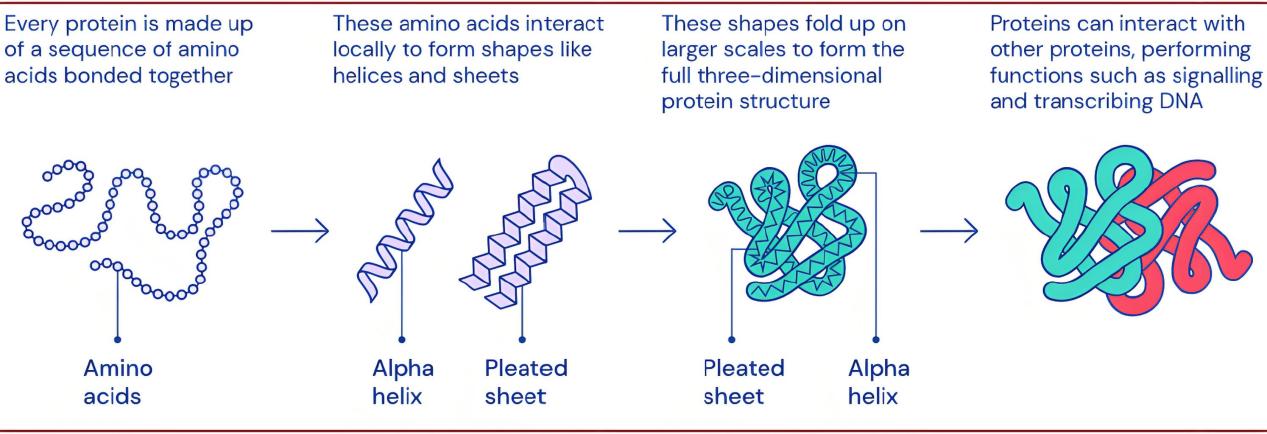
Figure 1. Protein folding process (Photo credit: Original).

The central focus of protein folding research lies in unraveling the process of how proteins progress from their primary sequence to intricate tertiary and higher-order structures, essentially deciphering the "folding blueprint." The thermodynamic hypothesis posited by Anfinsen underscores that the native state of a protein, under specific environmental conditions, represents its energetically most favorable conformation [1]. Consequently, the study of protein folding bifurcates into two principal avenues: firstly, the precise prediction of the three-dimensional structure of proteins at their minimum energy state, which is encompassed within the realm of protein folding structure prediction; secondly, the meticulous examination of the transition of proteins from a generic state to their native conformation, constituting the core domain of protein folding kinetics. By adopting this dual-track approach, we can gain a more comprehensive understanding of the intricate mechanisms underlying protein folding (figure 2).

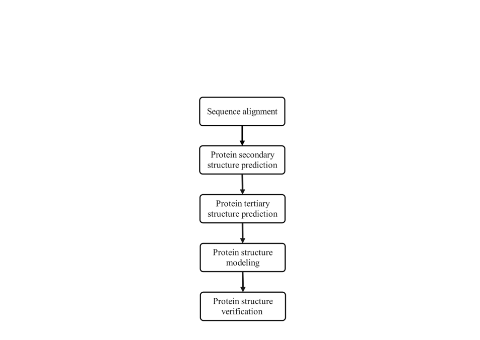
Figure 2. Flowchart of protein folding prediction (Photo credit: Original).

Protein models and their computational simulation

The problem of protein folding has been proven to be an NP-complete problem [2]. For instance, a protein consisting of merely 100 amino acids possesses approximately 10100 conformational states, assuming each amino acid adopts only 10 conformations. Even with the fastest supercomputer currently available, capable of 10 quadrillion operations per second, exploring the conformational space of such a protein would require approximately 10 to 16 seconds per conformation, leading to an estimated total time of approximately 3 x 1076 years to exhaustively search the entire conformational space. Consequently, exhaustive computational searches of protein conformational spaces are impractical, necessitating the research and design of more efficient algorithms for predicting the native structures of proteins [3]. To address this challenge, previous researches have proposed simplified models, which have now become instrumental in studying the fundamental properties of protein folding. In this paper, we introduce a particularly illustrative simplified model for protein folding: the HP lattice model, proposed by Dill et al. (HP Lattice Model) [4].

Dill and his team, drawing upon the characteristic feature of globular protein structures whereby "hydrophobic amino acid residues cluster together within the molecular interior, while hydrophilic amino acid residues are exposed to the aqueous interface," devised the HP lattice model. This model serves as a theoretical framework for comprehending protein folding. It simplifies the complexity of natural proteins by categorizing their twenty amino acids into two broad classes: hydrophobic (denoted as H) and hydrophilic (denoted as P), acknowledging that some amino acids may exhibit ambiguity in this binary classification. Based on this simplification, amino acid sequences are translated into sequences composed solely of H and P characters, forming a linear string that represents the protein chain. The folded configuration of such a sequence subsequently mirrors the three-dimensional structure of the protein.

As a free energy model, HP model focuses on simulating the natural conformation free energy, primarily governed by the interactions among hydrophobic amino acids, which tend to form a hydrophobic core surrounded by hydrophilic residues. The designation "lattice model" arises from the requirement that, in simulating protein chain folding, the HP chain must be mapped onto a two-dimensional orthogonal lattice network comprised of equally spaced horizontal and vertical gridlines, with each grid point spaced one unit apart. During the folding process, the following guidelines are adhered to ensure the legality of conformations:

Each monomer must occupy precisely one lattice site.

No lattice site can be simultaneously occupied by two or more monomers.

Monomers that were originally adjacent in the chain must remain adjacent (i.e., their Manhattan distance must be 1) after being mapped onto the lattice plane.

The HP model exhibits several salient features: firstly, it employs a uniform residue size standard; secondly, bond lengths are fixed and invariant; thirdly, it imposes strict lattice constraints on residue positions; and fourthly, it utilizes a simplified energy function to reduce computational complexity, thereby facilitating theoretical analysis and computational simulations. These characteristics render the HP model an efficacious tool for investigating protein folding mechanisms and predicting protein structures.

Two-dimensional HP model energy function. In the context of two-dimensional Euclidean space (Figure 3), we consider the problem of positioning amino acid monomers along a chain, labeled sequentially from 1 to N. When placed on a grid plane, each monomer i is assigned coordinates (xi, yi), where both xi and yi are integers. The HP lattice model adopts a simplistic energy function that solely accounts for the attractive interactions between hydrophobic amino acid monomers.

In a valid configuration, two H monomers are considered adjacent on the grid plane if their distance is unity, and they are not sequentially adjacent along the chain. Such a pair contributes a free energy of -1 to the system, while H-P and P-P pairs do not contribute any free energy. The formal energy function of the HP model can be expressed as:

\(E = \sum_{\begin{array}{r} i,j = 1 \\ i < j - 1 \end{array}}^{N}\sigma_{ij}\) (1)

\(\sigma_{ij} = \left\{ \begin{array}{r} - 1,\ i,j\ are\ H\ and\ their\ distance = 1 \\ 0,\ else \end{array} \right.\ \) (2)

From Equations (2.1) and (2.2), it is evident that the total sum of free energies across all interactions within a configuration represents the energy of that configuration. According to the laws of nature, protein folding invariably tends towards the configuration with the lowest energy. Therefore, the protein folding problem amounts to finding the lowest-energy configuration corresponding to a given HP chain.

Figure 3 presents the lowest-energy configuration for the protein chain HHHPPHHPPHHPHHPHPPHHP, with a corresponding minimum energy of E = -8.0. Notably, in this lowest-energy configuration, two parallel alpha-helical structures are formed.

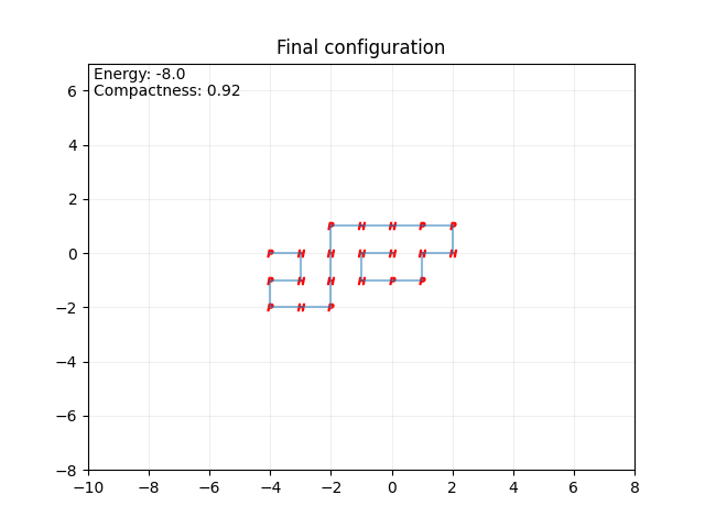
Figure 3. A protein conformation in the 2D HP model (Photo credit: Original).

Three-dimensional HP model energy function. In the three-dimensional (3D) context, the energy definition of the HP model remains unchanged, which is still the negative number of non-adjacent but spatially proximal hydrophobic amino acid (H) pairs along the chain. For the same protein sequence represented by an HP chain, the minimum energy value in the 3D form is significantly lower than that in the two-dimensional (2D) form. Figure 4 illustrates the 3D minimum energy configuration diagram and the protein folding simulation progress for the same protein sequence HP chain (HHHPPHHPPHHPHHPHPPHHP).

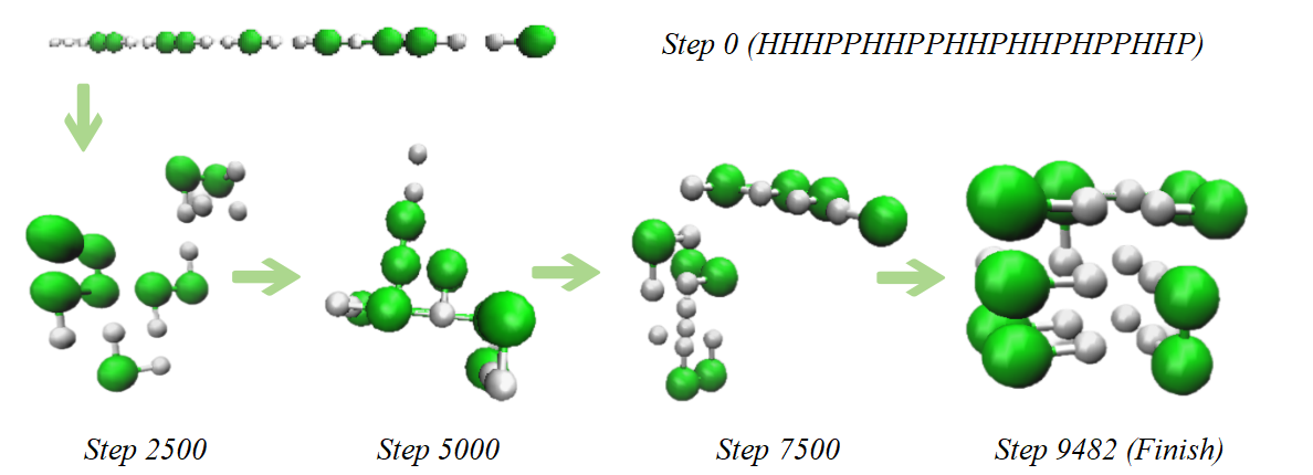
Figure 4. 3D Folding progress of the sequence.Green represents hydrophobic beads, white represents polar beads (Photo credit: Original).

In the 3D HP lattice model, a protein sequence is viewed as a chain of n balls, each of which has been assigned either a black or white color. For the i-th ball (i = 1, 2, ..., n), its centroid coordinates are denoted as (xi, yi, zi). Since it is a lattice model, the centroids of the balls must be placed on lattice points, thus the coordinates xi, yi, zi are all integers. The set of centroid coordinates (x1, y1, z1, ..., xn, yn, zn) at any given time represents a conformation. The problem of protein folding in this context involves adjusting the positions of these n balls in the lattice space such that all centroids reside on lattice points, the distance between the centroids of adjacent balls along the chain is 1, and the resulting conformation attains the minimum energy E. In this way, the protein folding problem in the 3D HP model can be mathematically formulated as follows:

\(Min(E)\) (3)

Also requires that:

\(\sqrt{{\left( x_{i} - x_{i + 1} \right)^{2}{+ \left( y_{i} - y_{i + 1} \right)}^{2} + \left( z_{i} - z_{i + 1} \right)}^{2}}\)= 1,i = 1,2,…,n-1 (4)

\(x_{i},\ y_{i},\ z_{i} \in Z\ \ \ \)i = 1,2,…,n (5)

Equation (2.4) ensures that the distance between the centroids of adjacent beads along the chain is 1. A conformation that satisfies the constraint conditions given by equations (2.4) and (2.5) is referred to as a legal conformation. It can be observed that equations (2.3) to (2.5) constitute a nonlinear constrained optimization problem.

Analysis and Application of Advanced Algorithms

The current exploration of protein folding primarily relies on molecular dynamics simulations and Monte Carlo simulations [5]. Specifically, molecular dynamics simulations excel in elucidating the dynamic evolution mechanisms of protein systems; in contrast, Monte Carlo methods offer a comprehensive examination of the overall thermodynamic processes within proteins. When dealing with high-resolution, all-atom protein models, the computational complexity soars, necessitating the meticulous consideration of the intricate interactions among a large number of atoms. Consequently, molecular dynamics simulations are constrained by computational limitations, typically capable of simulating protein folding processes only at the nanosecond scale, posing significant challenges for studies spanning longer time frames, such as microseconds to milliseconds. Monte Carlo simulations transcend these temporal constraints, effectively capturing folding behaviors across microseconds to milliseconds, and their processes are independent of a specific initial conformational structure, enabling unbiased exploration across a broader conformational space. In the following, we will delve into several classic algorithms that are widely employed in protein folding research.

Simulated annealing

Basic implementation of simulated annealing. The core of the algorithm lies in emulating the annealing process observed in the cooling and crystallization of solids or metallic solutions from high temperatures in thermodynamics. Drawing from Boltzmann's Principle of Order, the annealing process adheres strictly to the laws of thermodynamics, specifically the law of free energy minimization: In a closed system with constant heat exchange with its surroundings, spontaneous changes in the system's state occur in the direction of decreasing free energy, reaching equilibrium when the free energy attains its minimum value. The simulated annealing algorithm ingeniously substitutes the energy of a physical system with the objective function and the state of the system with the solution to a combinatorial minimization problem. In this context, the temperature in the physical system is transformed into a control parameter. Initially, the algorithm "melts" the solution space by setting a high initial temperature, then gradually "cools" it, simulating the random perturbations and trials within the system akin to the exploration in combinatorial minimization problems, until the system "solidifies" into an optimal and stable solution. This process encapsulates the transition from broad-scale search to refined optimization, effectively tackling complex optimization challenges.

Simulated annealing algorithm basically describes as follows:

Step 1: Select an arbitrary initial solution x0; set xi: =x0 and k: =0; establish the initial temperature t0: =tmax.

Step 2: If the internal loop termination condition is met at this temperature, proceed to Step 3; otherwise, randomly select a solution x j from the neighborhood N(xi) based on a certain transition distribution, and compute Δfij = f (x j) − f (xi). The replacement probability for xi is then determined as follows: if Δfij ≤0, then set xi: =x j. Otherwise, if exp (-Δfij / tk)> random (0,1), set xi: =x j. Repeat Step 2.

Step 3: Based on the progression described, the cooling schedule dictates that tk+1: =d(tk); k: =k+1. If the stopping condition is met, terminate the computation; otherwise, return to Step 2.

From the above steps, it is evident that the Simulated annealing algorithm operates as a double-loop algorithm, searching for an optimal solution at a given temperature and exploring the solution space for an optimal solution within a predefined accuracy range as the temperature cools down. Therefore, the transition distribution function, acceptance criterion, and cooling function can be considered the core components of this algorithm (Figure 5).

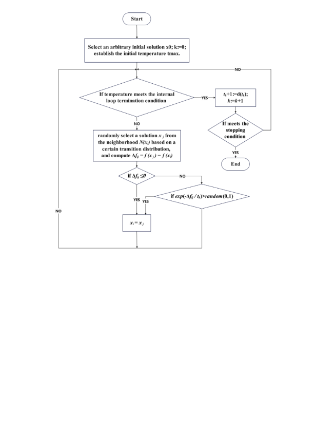
Figure 5. Flowchart of simulated annealing algorithm (Photo credit: Original).

Metropolis Principle. Although this method is relatively straightforward, it necessitates an extensive amount of sampling to yield more precise results, thereby leading to significant computational complexity. Physical systems tend to favor states of lower energy, yet thermal motion prevents them from precisely settling into the lowest-energy state. Given this scenario, by emphasizing the selection of states with significant contributions during sampling, a better outcome can be achieved more efficiently. In 1953, Metropolis and his colleagues proposed a sampling method that accepts new states with a certain probability. Its detailed description is as follows [6]:

After heating a metallic object to a certain temperature, the degrees of freedom of all its molecules in the state space D increase [7].

\(P_{r} = \left\{ \overline{E} = E(r) \right\} = \frac{1}{Z(T)}\exp\left\lbrack - \frac{E(r)}{k_{B}T} \right\rbrack\) (6)

Given two selected energies, E1 < E2, at the same temperature T, we have:

\(P_{r}\left\{ \overline{E} = E_{1} \right\} - P_{r}\left\{ \overline{E} = E_{2} \right\} = \frac{1}{Z(T)}\exp\left( - \frac{E_{1}}{k_{B}T} \right)\left\lbrack 1 - \exp\left( - \frac{E_{2} - E_{1}}{k_{B}T} \right) \right\rbrack\) (7)

Since:

\(\exp\left( - \frac{E_{2} - E_{1}}{k_{B}T} \right) < 1,\ \ \ \ \forall T > 0\) (8)

Therefore:

\(P_{r}\left\{ \overline{E} = E_{1} \right\} - P_{r}\left\{ \overline{E} = E_{2} \right\},\ \ \ \ \forall T > 0\) (9)

When the temperature is very high, the probability distribution given by Equation (3.1) results in approximately equal probabilities for each state, which are close to the average value of 1/\(|D|\), where \(|D|\) represents the number of states in the state space D. Furthermore, let rmin denote the state in D with the lowest energy, and since:

\(\frac{{\partial P}_{r}\left\{ \overline{E} = E(r) \right\}}{\partial T} = \frac{\exp\left\lbrack - \frac{E(r)}{k_{B}T} \right\rbrack}{Z(T)k_{B}T^{2}}\left\{ E(r) - \frac{\sum_{s \in D}^{}{E(s)\exp\left\lbrack - \frac{E(s)}{k_{B}T} \right\rbrack}}{Z(T)} \right\}\) (10)

Therefore:

\(\frac{{\partial P}_{r}\left\{ \overline{E} = E\left( r_{\min} \right) \right\}}{\partial T} < 0\) (11)

\(P_{r}\left\{ \overline{E} = E\left( r_{\min} \right) \right\} = \frac{1}{Z(T)}\exp\left\lbrack - \frac{E(r_{\min})}{k_{B}T} \right\rbrack = - \frac{1}{\left| D_{0} \right| + R}\) (12)

Furthermore, if \(D_{0}\) represents the set of all states with the lowest energy, then:

\(R = \sum_{s \in D;E(s) > E(r_{\min})}^{}{\exp\left\lbrack - \frac{E(s) - E(r_{\min})}{k_{B}T} \right\rbrack} \rightarrow 0,\ \ \ \ T \rightarrow 0\) (13)

Thus, as T approaches 0, we have:

\(P_{r}\left\{ \overline{E} = E\left( r_{\min} \right) \right\} \rightarrow \frac{1}{\left| D_{0} \right|},\ \ \ \ T \rightarrow 0\) (14)

From this, it can be concluded that as the temperature approaches 0, the probability of a molecule residing in the lowest energy state tends to 1. In other words, at very low temperatures (T → 0), the probability values for states with lower energies are higher, and in the limiting case, only the probability of the state with the lowest energy is non-zero.

For a combinatorial optimization problem,

\(\min\ \ \ \ z = f(x)\) \(s.t.\ \ \ \ g(x) \geq 0,\ \ \ \ x \in D\ \) (15)

When mapped to the annealing process of solids, we have:

\(P_{x}\left\{ \overline{Z} = Z(x) \right\} = \frac{1}{q(t)}\exp\left\lbrack - \frac{f(x)}{t} \right\rbrack\) (16)

In this equation, q(t) remains the normalization factor, corresponding to the exponential form \(\sum_{x\epsilon D}^{}{\exp\left\lbrack - \frac{f(x)}{t} \right\rbrack,\ }\)where the parameter kB is omitted without affecting the discussion. Upon this correspondence, simulated annealing should exhibit properties analogous to those of the genuine annealing process.

At low temperatures, the probability of x taking values that minimize z increases.

As the temperature approaches 0, the probability of f(x) converging to Zmin tends to 1.

The transition of the current solution towards the optimal solution is controlled by the change in the probability of states as the temperature decreases [8].

Genetic algorithm

Genetic Algorithm (GA) is a randomized search methodology evolved by drawing insights from the evolutionary principles observed in biological systems, namely, "survival of the fittest" and the genetic mechanisms of natural selection and reproduction. When applied to the research of protein folding, GA operates on a population of protein conformations. Through the processes of mutation, selection, and recombination among these conformations, the GA facilitates the evolution of protein structures, ultimately leading to the discovery of the optimal conformation [9, 10].

Utilizing genetic algorithms (GAs) to study protein folding in two-dimensional lattice models requires selecting an appropriate encoding scheme to represent the folding structures on orthogonal lattices, defining an appropriate energy function as the fitness function for the GA, and incorporating the Pull-Move operation, a form of local search, to enhance the algorithm. Specifically, the Pull-Move operation is introduced in sparse regions of the lattice within the standard GA framework.

Basic implementation of genetic algorithm. In addressing optimization problems with Genetic Algorithms (GAs), the optimal solution evolves gradually from a population of candidate solutions, each of which possesses a set of attributes that can mutate and alter. Traditionally, solutions are represented as binary strings composed of 0s and 1s, though alternative encoding schemes are also viable. The algorithm typically initiates with a randomly generated population and proceeds through iterative solutions. These altered candidate solutions are then utilized in the subsequent iteration of the algorithm. Typically, the algorithm halts when either the maximum number of iterations is reached or an optimal solution is identified. The fundamental flowchart of GA is illustrated in Figure 6.

The genetic representation of a candidate solution can be a set of binary digits or arrays of other types and structures, which essentially share the same convenience as binary representations in terms of having uniform lengths and facilitating easy alignment, thus simplifying crossover operations. Variable-length representations are feasible but complicate the crossover process.

Once the genetic representation and fitness function are established, GAs initialize a population of solutions and iteratively optimize them through mutation, crossover, and selection operations. As show in the figure 6.

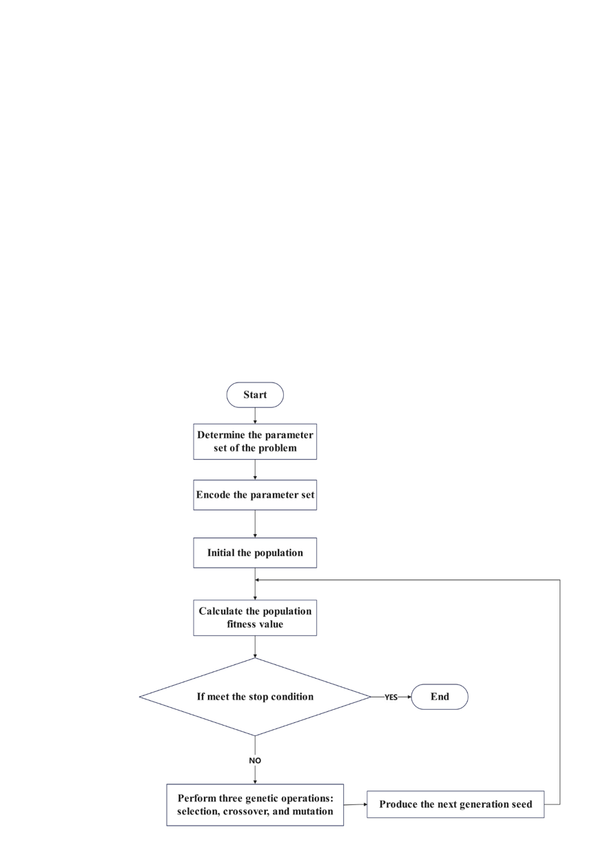
Figure 6. Basic flowchart of genetic algorithm (Photo credit: Original).

In genetic algorithms, the crossover operator possesses global search capabilities, serving as the primary operator, while the mutation operator exhibits local search capabilities, functioning as an auxiliary operator. The interplay between the crossover and mutation operators enhances the effectiveness of genetic algorithms, with the former complementing the latter.

Genetic algorithm used in the HP model. Step 1: Encoding.

Convert the input amino acid sequence into a sequence represented by "H" and "P." This encoding facilitates the subsequent genetic algorithm operations.

Step 2: Parameter Setting for the Algorithm.

Determine the population size, select the necessary genetic operators and their operational modes, probabilities, and the order of application. Additionally, establish the fitness function and stopping criteria.

Step 3: Initial Population Generation.

In this context, the initial population comprises solely of uncoiled conformations, where the chain follows a straight line path.

Step 4: Mutation.

For each individual in the population, a mutation operation is applied. Two types of mutations are employed in this context. The first mutation resembles a single Monte Carlo step mentioned in Section 3.1.1, adopting the same criteria for accepting a new conformation as the Monte Carlo method. The second mutation, termed Pull-Move, focuses on inducing curls in sparse regions of the grid. The specific definition is described as follows:

Consider the amino acid i at position (xi(t), yi(t)) at time t. Let L be adjacent to (xi+1(t), yi+1(t)) and diagonally adjacent to (xi(t), yi(t)), thus forming three corners of a square with L, (xi+1(t), yi+1(t)), and (xi(t), yi(t)). The fourth corner is denoted as C, as illustrated in Figure 7a.

The mutation can proceed only if C is empty or occupied by (xi-1(t), yi-1(t)). Initially, amino acid i is moved to L. If C = (xi-1(t), yi-1(t)), the move is completed, as shown in Figure 7b.

If C is empty, amino acid i-1 is then moved to C. If this results in a valid conformation, the movement stops, as depicted in Figure 7c.

Otherwise, for j ranging from i-2 down to 1, the movement rule is (xj(t+1), yj(t+1)) = (xj+2(t), yj+2(t)) until a valid conformation is achieved, as illustrated in Figure 7d.

For the endpoint n, amino acids n and n-1 are first moved to two free positions, followed by the remaining nodes from j = n-2 down to 1, using the same movement rule (xj(t+1), yj(t+1)) = (xj+2(t), yj+2(t)) until a valid conformation is reached. The operation for node 1 is analogous to that of node n.

It has been proven that the Pull-Move mutation is reversible and exhaustive. As show in the figure 7.

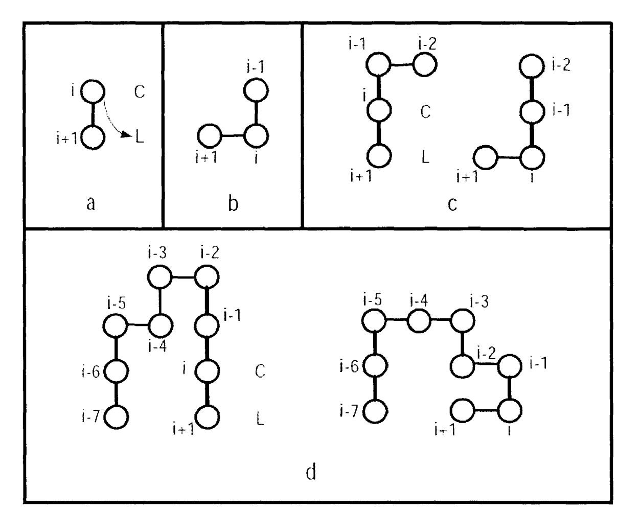
Figure 7. Curl operation Pull-move (Photo credit: Original).

Calculate the energy of the new conformation obtained through mutation, and then perform probabilistic selection of the new conformation based on the Monte Carlo method. If the energy of the new conformation is lower than that of the original conformation, the new conformation is directly accepted. If the energy of the new conformation is higher than that of the original conformation, instead of simply discarding it, which may lead to falling into a local extremum, a certain probability is applied to make the selection. The probability of accepting the new conformation is:

\(p = \left\{ \begin{array}{r} 1,\ \ \ \ E(c_{new}) \leq E(c) \\ \exp\left\lbrack - \frac{E(c_{new}) - E(c)}{t_{k}} \right\rbrack,\ \ \ \ E(c_{new}) > E(c) \end{array} \right.\ \) (17)

Wherein, \(t_{k}\) is a decreasing sequence with an initial value of t0=2, and it changes according to tk+1=0.97*\(t_{k}\). The iteration step changes every five steps.

Step 5: Crossover.

Perform crossover operations on the population. Each individual ci has a probability of being selected for crossover, which is calculated as \(p(c_{i}) = \frac{E_{i}}{\sum_{j = 1}^{N}E_{j}}\). For two individuals selected for crossover, randomly select a point in the sequence, and then connect the part behind the selected node in the first sequence to the part in front of the selected node in the second sequence, as shown in Figure 8. There are three methods to connect the two parts together, with the angles between the two chains being 0°, 90°, and 270°. An effective conformation is selected from these options. If no effective conformation can be obtained from all three methods, then select two other individuals for crossover. Once an effective conformation ck is obtained, calculate its energy Ek and compare it with the average energy \(\overline{E} = \frac{E_{i} + E_{j}}{2}\) of its parents. Select the new conformation according to the following probability:

\(p = \left\{ \begin{array}{r} 1,\ \ \ \ E_{k} \leq \overline{E_{ij}} \\ \exp\left\lbrack - \frac{\ E_{k} - \overline{E_{ij}}}{t_{k}} \right\rbrack,\ \ \ \ \ E_{k} > \overline{E_{ij}} \end{array} \right.\ \) (18)

If \(E_{k} \leq \overline{E_{ij}}\), conformation ck is directly accepted. Otherwise, selection is made based on probability. If Rnd < \(\exp\left\lbrack - \frac{\ E_{k} - \overline{E_{ij}}}{t_{k}} \right\rbrack\), conformation ck is accepted. This crossover operation is repeated until N-1 new conformations are generated. Additionally, the elitist strategy is adopted, where the best individual from each generation is directly copied to the next generation's population, thus generating a new population containing N individuals. As show in the figure 8.

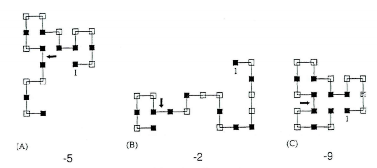
Figure 8. Crossover operation (Photo credit: Original).

Step 6: Determine if the stopping criterion is met.

The stopping criterion used here is to reach a certain number of iterations. If the criterion is not met, steps 4 and 5 are repeated continuously. If the criterion is met, the calculation stops, and the conformation with the lowest energy in the population is output, along with its energy and the sequence representing the folding path.

Generalized ensemble methods

The generalized ensemble method is one of the most commonly used approaches in protein folding research. Its fundamental idea lies in utilizing a non-Boltzmann distribution function to simulate free walks in the energy space, thereby enabling a more extensive exploration of the configuration space. Simultaneously, it can also calculate thermodynamic quantities of canonical ensembles across a wide range of temperatures, thereby facilitating further investigations into the thermodynamic processes of protein folding.

Relatively speaking, the Wang-Landau Monte Carlo method, which has evolved within the generalized ensemble approach in recent years, offers a more straightforward path to obtaining non-Boltzmann distribution functions. By iteratively adjusting a correction factor parameter F, this method automatically derives both the non-Boltzmann distribution function and the state density function of the protein system [11]. This approach not only facilitates the acquisition of non-Boltzmann distribution functions but also enables deeper exploration into the thermodynamic processes of protein folding through the analysis of the system's state density function.

As a widely used dynamic Monte Carlo method, the Wang-Landau algorithm possesses two major advantages:

By iteratively modifying the state density update modification factor f, it can rapidly obtain the state density of the system, demonstrating efficiency, intuitiveness, and simplicity. Furthermore, it facilitates the calculation of thermodynamic quantities in protein systems, enabling the study of the entire thermodynamic process of the system.

For systems with highly complex energy landscapes, such as protein systems, which possess numerous local energy minima, traditional Monte Carlo algorithms tend to get stuck in these local minima, making it difficult to effectively escape and reach the global energy minimum. In contrast, the Wang-Landau algorithm virtually eliminates this issue. By freely traversing the energy space, the Wang-Landau algorithm can effectively escape from local minima and locate the global energy minimum.

The fundamental aspect of the Wang-Landau algorithm lies in the utilization of an update modification factor f to determine the convergence precision of the algorithm. Specifically, at each given f, an appropriate spatial access movement method is employed to execute a certain number of Monte Carlo steps (abbreviated as MC sampling steps). Each MC move is accepted based on the following Metropolis criterion:

\(P(old \rightarrow new) = \min(1,\frac{g(E_{old})}{g(E_{new})}) = \min(1,e^{- \left\lbrack S\left( E_{new} \right) - S\left( E_{old} \right) \right\rbrack}\) (19)

Here, g(E) represents the density of states (DOS) explored by the algorithm. S(E) = ln g(E), which resembles the thermodynamic entropy value of protein systems, is primarily used in practical operations to avoid dealing with excessively large numbers. Evidently, initializing g(E) to 1 would result in every MC move being accepted, thereby yielding no useful information. The true ingenuity of the Wang-Landau algorithm lies in the fact that g(Ei) changes after every MC move, regardless of whether it is accepted or not:

\(g(E_{i}) = g(E_{i})*f\ (if\ accept\ the\ move\ i = new,otherwise\ i = old)\) (20)

Correspondingly, S(Ei) = S(Ei) + ln f, and the associated histogram count function H(Ei) is updated as H(Ei) = H(Ei) + 1. Once a sufficient number of MC steps have been completed (meeting a specific flattening criterion), the update modification factor f is decreased exponentially (typically using \(f = \sqrt{f}\)), and the Wang-Landau algorithm simulation iterates again. Finally, the simulation stops when ln f falls below a sufficiently small number. The basic flowchart is illustrated in Figure 9 below.

In the Wang-Landau algorithm, an initial value of f is typically chosen as e = 2.71828 [12]. If the initial value is too large, it will increase the error between the estimated density of states and the true density of states, affecting the convergence accuracy of the algorithm. Using the empirical initial value of 2.71828, even for systems with a large energy range, we can rapidly reach all energy values within an acceptable error range. At the end of the algorithm simulation, the value of f should approach 1, allowing the estimated density of states g(E) to closely approximate the true value. Furthermore, the typically set lower limit in the Wang-Landau algorithm is ln f = 10⁻⁸. As show in the figure 9.

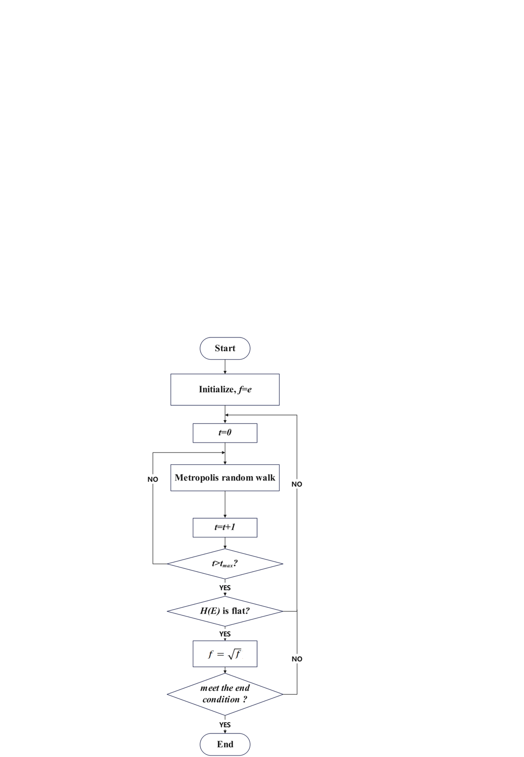
Figure 9. Basic flowchart of Wang-Landau algorithm (Photo credit: Original).

In the original algorithm, the flatness criterion for H(E) is generally set as: all values of H (Ei) are greater than 80% of their average value \(\overline{H}(E)\). However, this criterion appears to be overly strict, so it is also common to use a criterion where all H(Ei) reach a certain number (typically a small value such as 1). In some practical research applications, a flatness criterion based on a pre-defined maximum number of MC steps is also frequently employed.

The density of states g(E) obtained from the Wang-Landau algorithm is a relative value, which needs to be normalized for convenient calculation and comparison. If the reference density of states is \(\widetilde{g}(E)\), the normalization formula is as follows:

\(g(E) = \frac{g(E_{\min})}{\widetilde{g}(E_{\min})}\widetilde{g}(E)\) (21)

\(U(T) = \left\langle E \right\rangle_{T} = \frac{\sum_{E}^{}{Eg(E)e^{\frac{- E}{k_{B}T}}}}{\sum_{E}^{}{g(E)e^{\frac{- E}{k_{B}T}}}}\) (22)

\(C(T) = \frac{\partial U(T)}{\partial T} = \frac{\left\langle E^{2} \right\rangle_{T} - {\left\langle E \right\rangle^{2}}_{T}}{k_{B}T^{2}}\) (23)

\(F(T) = - k_{B}Tln(Z) = - k_{B}Tln(\sum_{E}^{}{g(E)e^{\frac{- E}{k_{B}T}}})\) (24)

Due to the simplicity and efficiency of the Wang-Landau algorithm, its application scope has been extended to clusters, magnetic systems, liquids, liquid crystals, spin glass models, as well as the protein folding issues we intend to study, among others.

Challenges

In the realms of bioinformatics and computational biology, genetic algorithms, simulated annealing algorithms, and generalized ensemble methods are potent tools for optimization. They are frequently employed in tasks like predicting protein structures, annotating functions, and modeling intricate biological systems. While these methods have proven their worth, they also come with notable limitations and challenges that students studying these fields should be aware of.

Genetic algorithms mimic natural evolution to search for optimal solutions. They excel at exploring large solution spaces but can sometimes converge too early to local optima instead of the global optimum. Additionally, fine-tuning parameters like the initial population, crossover and mutation rates, and the fitness function can be tricky and often relies on trial and error.

Simulated annealing algorithms, inspired by the physical process of annealing metals, aim to find the global optimum by gradually reducing the "temperature" of the system. However, they can be slow, especially as they approach the optimal solution, requiring careful balancing of the cooling rate to avoid getting stuck in local minima or wasting time.

Generalized ensemble methods, on the other hand, provide a flexible framework for describing complex systems. But their effectiveness hinges on knowing or accurately estimating the non-Boltzmann distribution function, which can be challenging or even impossible for complex biological systems.

In the future, to address these limitations, researchers must continue to explore novel algorithmic design ideas and improvement strategies. This includes leveraging machine learning techniques to optimize parameter settings, developing adaptive annealing strategies to enhance the efficiency of simulated annealing algorithms, and utilizing high-performance computing technologies to accelerate the simulation of complex systems. Additionally, deepening our understanding of the intrinsic mechanisms of biological systems and establishing more accurate mathematical models are crucial for improving the application effectiveness of these algorithms in the field of bioinformatics.

Conclusion

This paper has critically examined the principles of protein folding and the application of various optimization algorithms—namely, genetic algorithms, simulated annealing, and generalized ensemble methods—in simulating protein folding dynamics. These methods have been demonstrated to be effective in navigating the complex solution spaces inherent in protein structure prediction and other biological simulations. Genetic algorithms, with their evolutionary search mechanisms, are adept at exploring vast solution spaces but often face challenges related to premature convergence to local optima and parameter tuning. Simulated annealing algorithms, drawing inspiration from metallurgical annealing processes, offer a potential path to global optimum solutions but require careful management of cooling rates to avoid inefficiencies and local minima traps. Generalized ensemble methods provide a robust framework for simulating complex systems, although their effectiveness is contingent upon accurate estimations of non-Boltzmann distribution functions, which can be particularly challenging. Looking forward, there is a pressing need for further research to refine these methodologies and overcome the limitations currently facing them in bioinformatics applications. Future studies should focus on integrating advanced machine learning techniques to automate and optimize parameter settings, thereby enhancing the efficacy and efficiency of these algorithms. Additionally, the development of adaptive annealing strategies could significantly improve the performance of simulated annealing algorithms. High-performance computing technologies also hold the promise of accelerating the simulation of complex biological systems, enabling more detailed and expansive exploration of protein dynamics. Moreover, a deeper theoretical understanding of biological mechanisms and the establishment of more accurate mathematical models are vital for advancing the application of these computational techniques. By addressing these areas, future research can expand the capabilities of protein folding simulations, ultimately contributing to significant advancements in protein engineering and related fields.

References

[1]. Anfinsen, C. B. (1973). Principles that govern the folding of protein chains. Science, 181(4096), 223-230.
[2]. H. Xu, X. Zhu, Z. Zhao, X. Wei, X. Wang and J. Zuo, "Research of Pipeline Leak Detection Technology and Application Prospect of Petrochemical Wharf," 2020 IEEE 9th Joint International Information Technology and Artificial Intelligence Conference (ITAIC), Chongqing, China, 2020, pp. 263-271,
[3]. Zhu, X., Guo, C., Feng, H., Huang, Y., Feng, Y., Wang, X., & Wang, R. (2024). A Review of Key Technologies for Emotion Analysis Using Multimodal Information. Cognitive Computation, 1-27.
[4]. Dill, K. A., Bromberg, S., Yue, K., Chan, H. S., Ftebig, K. M., Yee, D. P., et al. (1995). Principles of protein folding — a perspective from simple exact models. Protein Science.
[5]. Zhang, Y., Zhao, H., Zhu, X., Zhao, Z., & Zuo, J. (2019, October). Strain Measurement Quantization Technology based on DAS System. In 2019 IEEE 3rd Advanced Information Management, Communicates, Electronic and Automation Control Conference (IMCEC) (pp. 214-218). IEEE.
[6]. Hansmann, U. H. E., & Okamoto, Y. (1994). Comparative study of multicanonical and simulated annealing algorithms in the protein folding problem. Physica A: Statistical Mechanics and its Applications, 212(3–4), 415-437.
[7]. Zhu, X., Huang, Y., Wang, X., & Wang, R. (2023). Emotion recognition based on brain-like multimodal hierarchical perception. Multimedia Tools and Applications, 1-19.
[8]. Metropolis, N., Rosenbluth, A. W., Rosenbluth, M. N., Teller, A. H., & Teller, E. (1953). Equation of state by fast computing machines. Journal of Chemical Physics, 21(6), 1087-1092.
[9]. Zhu, X., Zhang, Y., Zhao, Z., & Zuo, J. (2019, July). Radio frequency sensing based environmental monitoring technology. In Fourth International Workshop on Pattern Recognition (Vol. 11198, pp. 187-191). SPIE.
[10]. Shatabda, S., Newton, M. H., Rashid, M. A., & Sattar, A. (2013). An efficient encoding for simplified protein structure prediction using genetic algorithms. IEEE.
[11]. Wang R., Zhu J., Wang S., Wang T., Huang J., Zhu X. Multi-modal emotion recognition using tensor decomposition fusion and self-supervised multi-tasking. International Journal of Multimedia Information Retrieval, 2024, 13(4): 39.
[12]. Singh, P., Sarkar, S. K., & Bandyopadhyay, P. (2011). Understanding the applicability and limitations of Wang–Landau method for biomolecules: Met-enkephalin and trp-cage. Chemical Physics Letters, 514(4–6), 357-361.
Cite this article
Yin,Y. (2024). Comprehensive Analysis and Application Research of Advanced Computational Algorithms in Protein Folding Simulations. Theoretical and Natural Science,65,141-155.
Data availability
The datasets used and/or analyzed during the current study will be available from the authors upon reasonable request.
Disclaimer/Publisher's Note
The statements, opinions and data contained in all publications are solely those of the individual author(s) and contributor(s) and not of EWA Publishing and/or the editor(s). EWA Publishing and/or the editor(s) disclaim responsibility for any injury to people or property resulting from any ideas, methods, instructions or products referred to in the content.
About volume
Volume title: Proceedings of ICBioMed 2024 Workshop: Computational Proteomics in Drug Discovery and Development from Medicinal Plants
© 2024 by the author(s). Licensee EWA Publishing, Oxford, UK. This article is an open access article distributed under the terms and
conditions of the Creative Commons Attribution (CC BY) license. Authors who
publish this series agree to the following terms:
1. Authors retain copyright and grant the series right of first publication with the work simultaneously licensed under a Creative Commons
Attribution License that allows others to share the work with an acknowledgment of the work's authorship and initial publication in this
series.
2. Authors are able to enter into separate, additional contractual arrangements for the non-exclusive distribution of the series's published
version of the work (e.g., post it to an institutional repository or publish it in a book), with an acknowledgment of its initial
publication in this series.
3. Authors are permitted and encouraged to post their work online (e.g., in institutional repositories or on their website) prior to and
during the submission process, as it can lead to productive exchanges, as well as earlier and greater citation of published work (See
Open access policy for details).