1. Introduction

Earthquakes are the products of the earth's interior tectonic movements and area natural phenomena. There are about 5 million earthquakes worldwide each year. The vast majority, which accounts for about 99% of the total number of earthquakes in a year, are small enough to be measured only with susceptible instruments. Moreover, the remaining 1% is the severe earthquake that people can feel and are capable of causing severe damage, of which the average annual occurrence is about 18 times in the whole world [1]. The earthquake has brought disasters to society, causing different degrees of personal injury and economic loss. At 14:28 on May 12, 2008, a strong earthquake of magnitude 8.0 on the Richter scale occurred in Wenchuan County, Sichuan Province, China, which was the largest, most destructive earthquake since the founding of the People's Republic of China, causing huge losses to people's lives and property safety [2,3]. Highways, bridges, tunnels, and other essential infrastructure were seriously damaged during the earthquake. The damage to buildings is mainly due to the strong vibration of the ground caused by seismic waves, resulting in the collapse of ground buildings.

Therefore, to understand the earthquake's impact on buildings or how the earthquake destroyed the buildings, we decided to find out the characteristics of the two-story building under the effect of an earthquake. We simulated the earthquake by making two different two-story frames under an applied and impulsive load. As a result, we managed to find the displacement of the structures with and without damping.

2. Procedure

2.1. Challenge 1

2.1.1. Formulate the equation of motion. The mass of each story of the idealized two-story frame is m=50kips/g, which is

\( \frac{50kips}{386 in/{s^{2}}}=0.130kips∙\frac{{s^{2}}}{in} \) (1)

for each story. Moreover, the stiffness for each story is k=15.77 kips/in (k/2 for each column). To set up the equation of motion for a multiple-degree-of-freedom system (two-degree of freedom for this project), the mass and stiffness properties have to be derived as a matrix [4]. Therefore, the mass matrix and stiffness matrix for this project is

\( m=[\begin{matrix}m & 0 \\ 0 & m \\ \end{matrix}]=[\begin{matrix}0.13 & 0 \\ 0 & 0.13 \\ \end{matrix}] \) (2)

and

\( k=[\begin{matrix}{k_{1}}+{k_{2}} & -{k_{2}} \\ -{k_{2}} & {k_{2}} \\ \end{matrix}]=[\begin{matrix}31.54 & -15.77 \\ -15.77 & 15.77 \\ \end{matrix}] \) (3)

respectively. Since the equation of motion for the undamped multiple-degree-of-freedom system with no applied force is

\( m\ddot{u}+ku=0 \) (4)

in our case, it can be set up as

\( [\begin{matrix}0.13 & 0 \\ 0 & 0.13 \\ \end{matrix}][\begin{matrix}{\ddot{u}_{1}} \\ {\ddot{u}_{2}} \\ \end{matrix}]+[\begin{matrix}31.54 & -15.77 \\ -15.77 & 15.77 \\ \end{matrix}][\begin{matrix}{u_{1}} \\ {u_{2}} \\ \end{matrix}]=[\begin{matrix}0 \\ 0 \\ \end{matrix}] \) (5)

when plugging the mass matrix and stiffness matrix in.

2.1.2. Compute natural frequencies ( \( {ω_{1}} \) and \( {ω_{2}} \) ) and the corresponding mode shapes ( \( {ϕ_{1}} and {ϕ_{2}} \) ). Multi-degree freedom systems can do free vibration at specific natural frequencies [1]. For the equation of motion of multiple-degree of freedom system (1-4), assume the displacement response as a function of time (t)

\( u(t)=\hat{u}sin{(ωt+θ)} \) (6)

where \( \hat{u} \) is the modal component. Then the second derivative of \( u(t) \) is

\( \ddot{u}(t)=-{ω^{2}}\hat{u}sin{(ωt+θ)} \) , (7)

So, it can be written down as

\( \ddot{u}=-{ω^{2}}u \) (8)

Then apply this equation to the equation of motion, we can get

[ \( k-{ω^{2}}m \) ] \( u=0 \) (9)

Moreover, the displacement cannot always be 0 because of the arbitrary loading. Thus, the equation can be written as

\( |k-{ω^{2}}m|=0 \) , (10)

which is called the frequency equation. Then plug the mass and stiffness matrix in the frequency equation, and another equation concerning \( ω \) can be obtained as

\( 0.0169{ω^{4}}-6.1503{ω^{2}}+248.6929=0 \) , (11)

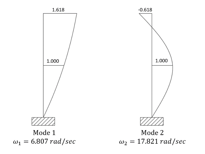
From which there are two opposing and two positive values for \( ω \) . Since the natural frequencies cannot be less than 0, the negative results must be neglected, so the natural frequencies for this structure are \( \begin{cases} \begin{array}{c} {ω_{1}}=6.807 rad/s \\ {ω_{2}}=17.821 rad/s \end{array} \end{cases} \) . When free vibration at a natural frequency, the structure will remain a fixed shape called a mode shape. For the first mode where \( {ω_{1}}=6.807 rad/s \) , assume u₁=1. Then the equation can obtain the mode shape for the first mode.

\( [\begin{matrix}25.516 & -15.77 \\ -15.77 & 9.746 \\ \end{matrix}][\begin{matrix}{u_{1}}=0 \\ {u_{2}} \\ \end{matrix}]=[\begin{matrix}0 \\ 0 \\ \end{matrix}] \) (12)

and \( {ϕ_{1}}= [\begin{matrix}1 \\ 1.618 \\ \end{matrix}] \) . Similarly, for the second mode where \( {ω_{2}}=17.821 rad/s \) , the mode shape can be obtained by

\( [\begin{matrix}-9.746 & -15.77 \\ -15.77 & -25.516 \\ \end{matrix}][\begin{matrix}{u_{1}}=0 \\ {u_{2}} \\ \end{matrix}]=[\begin{matrix}0 \\ 0 \\ \end{matrix}] \) (13)

and \( {ϕ_{2}}= [\begin{matrix}1 \\ -0.618 \\ \end{matrix}] \) . In addition,

\( Φ=[\begin{matrix}{ϕ_{1}} & {ϕ_{2}} \\ \end{matrix}]=[\begin{matrix}1 & 1 \\ 1.618 & -0.618 \\ \end{matrix}] \) (14)

which is the mode shape matrix. The mode shapes of the structure and the corresponding natural frequencies are shown in Figure 1 below.

2.2. Determine the undamped displacement response of the structure with the initial condition.

For any modal component \( {\hat{u}_{n}} \) , we can write

\( {\hat{u}_{n}}={ϕ_{n}}{Y_{n}} \) , (15)

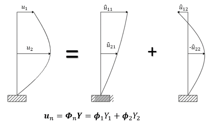
where \( {Y_{n}} \) is the \( {n^{th}} \) normal coordinate (or modal coordinate). Then the total displacement through the modal superposition is

\( u=\sum _{n=1}^{N}{ϕ_{n}}{Y_{n}}=ΦY \) , (16)

where N is the degree of freedom. The total displacement calculated by the modal superposition method can be shown in Figure 2.

With equation (16), we use orthogonality to evaluate Y. Since

\( u=ΦY \) , (17)

we multiply both sides of the equation by \( ϕ_{n}^{T}m \) :

\( ϕ_{n}^{T}mu=ϕ_{n}^{T}m{ϕ_{1}}{Y_{1}}+ϕ_{n}^{T}m{ϕ_{2}}{Y_{2}}+…+ϕ_{n}^{T}m{ϕ_{n}}{Y_{n}}+…+ϕ_{n}^{T}m{ϕ_{N}}{Y_{N}} \) , (18)

Where \( ϕ_{n}^{T} \) is the matrix transpose of \( {ϕ_{n}} \) . Then due to the orthogonality condition:

\( \begin{cases} \begin{array}{c} ϕ_{m}^{T}m{ϕ_{n}}=0,      m≠n \\ ϕ_{m}^{T}m{ϕ_{n}}={M_{n}},    m=n  \end{array} \end{cases} \) , (19)

And similarly for stiffness.

\( \begin{cases} \begin{array}{c} ϕ_{m}^{T}k{ϕ_{n}}=0,      m≠n \\ ϕ_{m}^{T}k{ϕ_{n}}={K_{n}},    m=n  \end{array} \end{cases} \) , (20)

Other terms vanish where \( {M_{n}} and {K_{n}} \) are scalars are called general mass and general stiffness. Consequently, we have

\( ϕ_{n}^{T}mu=ϕ_{n}^{T}m{ϕ_{n}}{Y_{n}} \) , (21)

which means

\( {Y_{n}}=\frac{ϕ_{n}^{T}mu}{ϕ_{n}^{T}m{ϕ_{n}}} \) (22)

Therefore, the general mass must be obtained for calculating the modal coordinate. The equation can calculate the general mass for the first mode shape.

\( {M_{1}}=ϕ_{1}^{T}m{ϕ_{1}}=[\begin{matrix}1 & 1.618 \\ \end{matrix}][\begin{matrix}0.13 & 0 \\ 0 & 0.13 \\ \end{matrix}][\begin{matrix}1 \\ 1.618 \\ \end{matrix}] \) (23)

Then we can get our first general mass \( {M_{1}}=0.4703 kips∙s/{in^{2}} \) . Similarly, the second general mass \( {M_{2}}=0.1797 kips∙s/{in^{2}} \) .

Last step before we calculate the modal coordinate is to achieve modal equations of motion using orthogonality. Therefore, for each modal equation of motion (4), the multi-degree-of-freedom problem becomes a single-degree-of-freedom problem [5]. For the multi-degree of freedom equation of motion, we now have \( u=ΦY \) and

\( \ddot{u}=Φ\ddot{Y} \) (24)

(Mode shapes do not change through time). Then the equation of motion can be written as

\( mΦ\ddot{Y}+kΦY=0 \) (25)

Multiply both sides by \( ϕ_{n}^{T} \) ; we can get

\( ϕ_{n}^{T}mΦ\ddot{Y}+ϕ_{n}^{T}kΦY=0 \) (26)

And due to the orthogonality, the equation of motion becomes

\( ϕ_{n}^{T}m{ϕ_{n}}{\ddot{Y}_{n}}+ϕ_{n}^{T}k{ϕ_{n}}{Y_{n}}=0 \) , (27)

where \( ϕ_{n}^{T}m{ϕ_{n}}{\ddot{Y}_{n}} \) and \( ϕ_{n}^{T}k{ϕ_{n}}{Y_{n}} \) are general mass and general stiffness, respectively, which are both scalars as well as \( {\ddot{Y}_{n}} \) and \( {Y_{n}} \) . Therefore, we have the single degree of freedom equation of motion

\( {M_{n}}{\ddot{Y}_{n}}+{K_{n}}{Y_{n}}=0 \) (28)

for each mode. For this equation, we use a second-order ordinary differential equation, and we can get

\( {Y_{n}}(t)=Asin{ω_{n}}t+Bcos{ω_{n}}t \) and \( {\dot{Y}_{n}}(t)=A{ω_{n}}cos{ω_{n}}t-B{ω_{n}}sin{ω_{n}}t \) (29)

And according to the initial condition, which is when t=0,

\( \begin{cases} \begin{array}{c} {Y_{n}}(0)=B \\ {\dot{Y}_{n}}(0)=A{ω_{n}} \end{array} \end{cases} \) (30)

Thus,

\( {Y_{n}}(t)=\frac{{\dot{Y}_{n}}(0)}{{ω_{n}}}sin{ω_{n}}t+{Y_{n}}(0)cos{ω_{n}}t \) (31)

Then plug the initial condition given: \( \begin{cases} \begin{array}{c} u(0)=[\begin{matrix}1 \\ 0 \\ \end{matrix}] \\ \dot{u}(0)=[\begin{matrix}0 \\ 2 \\ \end{matrix}] \end{array} \end{cases} \) in the equations:

\( \begin{cases} \begin{array}{c} {Y_{n}}(0)=\frac{ϕ_{n}^{T}mu(0)}{{M_{n}}} \\ {\dot{Y}_{n}}(0)=\frac{ϕ_{n}^{T}m\dot{u}(0)}{{M_{n}}} \end{array} \end{cases} \) \( \begin{matrix}(32) \\ (33) \\ \end{matrix} \)

we can get

\( \begin{cases} \begin{array}{c} {Y_{1}}(0)=\frac{ϕ_{1}^{T}mu(0)}{{M_{1}}}=0.2764 \\ {Y_{2}}(0)=\frac{ϕ_{2}^{T}mu(0)}{{M_{2}}}=0.7234 \end{array} \end{cases} \) \( \begin{matrix}(34) \\ (35) \\ \end{matrix} \)

and

\( \begin{cases} \begin{array}{c} {\dot{Y}_{1}}(0)=\frac{ϕ_{1}^{T}m\dot{u}(0)}{{M_{1}}}=0.8945 \\ {\dot{Y}_{2}}(0)=\frac{ϕ_{2}^{T}m\dot{u}(0)}{{M_{2}}}=-0.8972 \end{array} \end{cases} \) . \( \begin{matrix}(36) \\ (37) \\ \end{matrix} \)

Next, we plug \( \begin{cases} \begin{array}{c} {Y_{1}}(0)=0.2764 \\ {Y_{2}}(0)=0.7234 \end{array} \end{cases} \) and \( \begin{cases} \begin{array}{c} {\dot{Y}_{1}}(0)=0.8945 \\ {\dot{Y}_{2}}(0)=-0.8972 \end{array} \end{cases} \) in equation (1-31); we can get our equation of \( {Y_{n}}(t) \) :

\( \begin{cases} \begin{array}{c} {Y_{1}}(t)=0.1314sin6.807t+0.2764cos6.807t \\ {Y_{2}}(t)=-0.0502sin17.821t+0.7234cos17.821t \end{array} \end{cases} \) \( \begin{matrix}(38) \\ (39) \\ \end{matrix} \)

Finally, according to the modal superposition method, the ultimate undamped displacement response of the structure is

\( u=[\begin{matrix}1 \\ 1.618 \\ \end{matrix}](0.1314sin6.807t+0.2764cos6.807t)+[\begin{matrix}1 \\ -0.618 \\ \end{matrix}](-0.0502sin17.821t+0.7234cos17.821t) \) . (40)

Consequently, the displacement for the first floor is:

\( {u_{1}}=0.1314sin6.807t+0.2764cos6.807t-0.0502sin17.821t+0.7234cos17.821t \) (41)

Moreover, the second floor is:

\( {u_{2}}=0.2208sin6.807t+0.4644cos6.807t+0.031sin17.821t-0.4471cos17.821t \) (42)

2.3. The displacements as functions of time when the undamped system is subjected to a suddenly applied force at the first floor: \( {p_{1}}(t)={p_{0}} \) , where \( t≥0 \) and \( {p_{0}}=10 kips \) , and the shear force for the second story.

Since we have obtained the single degree of freedom equation of motion with no applied load (4), the equation of motion with applied load is

\( {M_{n}}{\ddot{Y}_{n}}+{K_{n}}{Y_{n}}={P_{n}}(t) \) (43)

Moreover, since only the first story is subjected to a force, the equation of motion for the second story remains the same as equation (1-4). The position of the applied force is shown in Figure 3 below.

Do the second-order ordinary differential equation to the first-floor equation of motion, we can get

\( {Y_{1}}(t)=Asin{ω_{1}}t+Bcos{ω_{1}}t+\frac{{p_{0}}}{{K_{1}}} \) (44)

and

\( {\dot{Y}_{1}}(t)=A{ω_{1}}cos{ω_{1}}t-B{ω_{1}}sin{ω_{1}}t \) (45)

Then we use the initial condition like before we can get

\( \begin{cases} \begin{array}{c} A=\frac{{\dot{Y}_{1}}(0)}{{ω_{1}}}  \\ B={Y_{1}}(0)-\frac{{p_{0}}}{{K_{1}}} \end{array} \end{cases} \) , \( \begin{matrix}(46) \\ (47) \\ \end{matrix} \)

which means we have to solve for the general stiffness first. For the first and second stories, the general stiffness is

\( {K_{1}}=[\begin{matrix}1 & 1. \\ \end{matrix}618][\begin{matrix}31.54 & -15.77 \\ -15.77 & 15.77 \\ \end{matrix}][\begin{matrix}1 \\ 1.618 \\ \end{matrix}]=21.793 kips/in \) (48)

and

\( {K_{2}}=[\begin{matrix}1 & -0. \\ \end{matrix}618][\begin{matrix}31.54 & -15.77 \\ -15.77 & 15.77 \\ \end{matrix}][\begin{matrix}1 \\ -0.618 \\ \end{matrix}]=25.517 kips/in \) (49)

Respectively. So,

\( \begin{cases} \begin{array}{c} A=\frac{0.8945}{6.807}=0.1314 \\ B=0.2764-\frac{10}{21.793}=0.1825 \end{array} \end{cases} \) (50)

and

\( {Y_{1}}(t)=0.1314sin6.807t-0.1825cos6.807t+0.458 \) (51)

Since the second story remains in the same condition, the displacement response now becomes

\( u=[\begin{matrix}1 \\ 1.68 \\ \end{matrix}](0.1314sin6.807t-0.1825cos6.807t+0.458)+[\begin{matrix}1 \\ -0.618 \\ \end{matrix}](-0.0502sin17.821t+0.7234cos17.821t) \) (52)

And the displacement for the first and second stories is

\( {u_{1}}(t)=0.1314sin6.807t-0.1825cos6.807t+0.458 \)

\( -0.0502sin17.821t+0.7234cos17.821t \) (53)

and

\( {u_{2}}(t)=0.2126sin6.807t-0.2953cos6.807t+0.741 \)

\( +0.031sin17.821t-0.4471cos17.821t \) (54)

respectively.

For the story shear in the second story,

\( {V_{2}}=k({u_{2}}-{u_{1}}) \) , (55)

where k=15.77 kips/in is the stiffness for the second story. The relative displacement for the second story is

\( ({u_{2}}-{u_{1}})=0.0812sin6.807t-0.1128cos6.807t+0.283+0.0812sin17.821t-1.1705cos17.821t \) (56)

Therefore, the story shear on the second floor is

\( {V_{2}}=1.281sin6.807t-1.779cos6.807t+4.463+1.281sin17.821t-18.459cos17.821t \) (57)

2.4. Assume there is stiffness-proportional damping ( \( {C_{n}}=α{K_{n}} \) ) with a modal damping ratio corresponding to the first mode \( {ξ_{1}}=0.05 \) .

For the damped multi-degree of freedom equation of motion, we must assume that the damping can satisfy the orthogonality as well, which means

\( \begin{cases} \begin{array}{c} ϕ_{m}^{T}c{ϕ_{n}}={C_{n}} ,m=n \\ ϕ_{m}^{T}c{ϕ_{n}}=0 ,m≠n \end{array} \end{cases} \) . \( \begin{matrix}（58） \\ （59） \\ \end{matrix} \)

Then for the damped multi-degree of freedom equation of motion

\( m\ddot{u}+c\dot{u}+ku=0 \) , (60)

we can pre-multiply both sides by \( ϕ_{n}^{T} \) and get

\( ϕ_{n}^{T}mΦ\ddot{Y}+ϕ_{n}^{T}cΦ\dot{Y}+ϕ_{n}^{T}kΦY=0 \) . (61)

Due to the damping orthogonality, we just assumed the equation of motion could be uncoupled into

\( {M_{n}}{\ddot{Y}_{n}}+{C_{n}}{\dot{Y}_{n}}+{K_{n}}{Y_{n}}=0 \) , (62)

which is the single degree of freedom equation. And in a single degree of freedom problems

\( {C_{n}}=2{ξ_{n}}{ω_{n}}{M_{n}} \) , (63)

where \( {ξ_{n}} \) is the damping ratio. Therefore,

\( {C_{1}}={2{ξ_{1}}ω_{1}}{M_{1}}=0.3201 \) . (64)

And according to stiffness-proportional damping

\( {C_{n}}=α{K_{n}} \) , (65)

the coefficient \( α \) can be solved by

\( α=\frac{{C_{1}}}{{K_{1}}} \) , (66)

which equals 0.0147. Then we can solve the second damping by

\( {C_{2}}=α{K_{2}} \) , (67)

which is 0.375. Moreover, according to equation (63), the second damping ratio is

\( {ξ_{2}}= \) \( \frac{{C_{2}}}{{2ω_{2}}{M_{2}}}=0.058 \) . (68)

2.5. Challenge 2

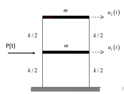
2.5.1. Derive the mass matrix(m) and the stiffness matrix(k). The question is a two-story frame. The mass of the top floor is m=10 \( \frac{kips∙{s^{2}}}{in} \) , and the mass of the ground floor is 2m=20 \( \frac{kips∙{s^{2}}}{in} \) . Therefore, the stiffness for the top floor is k=500kips/in, and the stiffness for the ground floor is 2k=1000kips/in. After having these data, we can derive them as a matrix. For example, we know the equation for the mass matrix \( [\begin{matrix}2m & 0 \\ 0 & m \\ \end{matrix}] \) and the stiffness matrix \( [\begin{matrix}{k_{1}}+{k_{2}} & -{k_{2}} \\ -{k_{2}} & {k_{2}} \\ \end{matrix}] \) . Therefore, we can get the mass matrix \( [\begin{matrix}20 & 0 \\ 0 & 10 \\ \end{matrix}] \) and the stiffness matrix \( [\begin{matrix}1500 & -500 \\ -500 & 500 \\ \end{matrix}] \) .

2.5.2. Compute the two natural frequencies \( ω \) and mode shapes. The natural frequency is when a structural system is excited to generate motion, the specific frequency is determined only by the nature of the system itself. We use the mass matrix and the stiffness matrix to get the equation of motion [4]. The equation of motion of multiple degrees of freedom system is

\( m\ddot{u}+ku=0 \) .(69)

Similarly, the acceleration \( \ddot{u} \) equals \( -{ω^{2}}\hat{u}sin{(ωt+θ)} \) . Then it can be written down as \( -{ω^{2}}u \) . After that, we can get

[ \( k-{ω^{2}}m \) ] \( \hat{u}=0 \) ,(70)

as the frequency equation and the displacement is what we are trying to compute. Thus, it cannot always be 0. So, the equation can be written as

\( |k-{ω^{2}}m| \) . (71)

That is the equation that will help us find the natural frequency. Then we can plug the mass and stiffness matrix which have been obtained in the first step; the equation is

[ \( k-{ω^{2}}m \) ] \( =[\begin{matrix}1500-20{ω^{2}} & -500 \\ -500 & 500-10{ω^{2}} \\ \end{matrix}] \) ,(72)

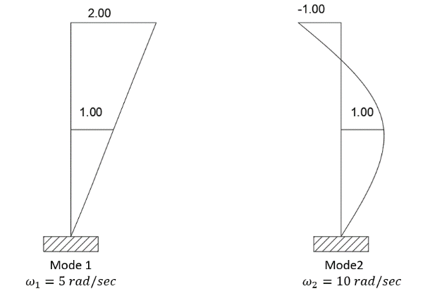
which can be calculated to \( 200{ω^{4}}-25000{ω^{2}}+500000 \) , and make it equal to 0. Then we can get four values for natural frequencies, which are -5, -10, +5, and +10. The natural frequencies cannot be harmful, so the natural frequencies for this structure are \( {ω_{1}}=5 \) rad/s \( { and ω_{2}}=10 \) rad/s. For \( {ω_{1}}=5 \) rad/s, we can get the first mode shape

\( {ϕ_{1}}=[\begin{matrix}1 \\ 2 \\ \end{matrix}] \) (73)

by assuming \( {u_{1}}=1 \) . Similarly, the \( {ϕ_{2}} \) can be computed in the same way. For the natural frequency of the second mode shape \( {, ω_{2}}=10 \) rad/s. The first and second mode shapes are shown in Figure 4.

\( {ϕ_{2 }}=[\begin{matrix}-1 \\ 1 \\ \end{matrix}] \) (74)

2.5.3. Determine the displacements \( {v_{1}} \) and \( { v_{2}} \) of the structure as a function of time. Firstly, we plan to find the general mass by using the equation

\(  ϕ_{m}^{T}m{ϕ_{n}}={M_{n}} \) ,(75)

the mass matrix \( [\begin{matrix}20 & 0 \\ 0 & 10 \\ \end{matrix}] \) and the \( {ϕ_{1}} \) matrix \( [\begin{matrix}1 \\ 2 \\ \end{matrix}] \) are for \( { M_{1}} \) , so the equation is

\( {M_{1}}=[\begin{matrix}1 & 2 \\ \end{matrix}][\begin{matrix}20 & 0 \\ 0 & 10 \\ \end{matrix}][\begin{matrix}1 \\ 2 \\ \end{matrix}] \) =60 \( kips∙s/{in^{2}} \) . (76)

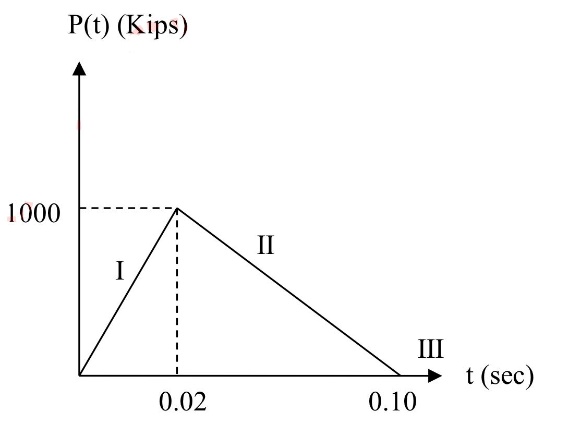
Similarly, we can get \( {M_{2}} \) using the mass matrix \( [\begin{matrix}20 & 0 \\ 0 & 10 \\ \end{matrix}] \) and the \( {ϕ_{2 }} \) matrix \( [\begin{matrix}1 \\ -1 \\ \end{matrix}] \) . So, \( { M_{1}} \) the is 60 \( kips∙s/{in^{2}} \) and the \( {M_{2}} \) is 30 \( kips∙s/{in^{2}} \) . Secondly, we need to determine the p(t) expression for each phase. In phase 1, from the graph, we can get p(0) is equal to 1000kips, and the period in phase 1 t(1) is equal to 0.02sec. Then we can determine the equation for the p(t) is equal to \( { P_{0}}×(\frac{t}{{t_{1}}} \) ). We plug the value of p(0) and t(1) into the equation, so

p(t) \( = \) 50000t.(77)

For phase 2 from the graph, we can regard this part of the function as a linear function

y=kx+b. (78)

Then we can get

k \( =\frac{0-P(0)}{0.1-{t_{1}}} \) (79)

and plug P(0)=1000Kips, t1=0.02sec into the equation. Therefore, we can get \( k=-12500 \) . After that, we can get b=-0.01k. So, the value of b is 1250, and

p(t) \( =- \) 12500t+1250.(80)

For phase 3, there is no p(t) on the graph, so the value equals 0.

Thirdly, we should use the Duhamel integral to express the function of displacements by time. At first, the equation for the Duhamel integral is

\( v(t)=\int _{{t_{1}}}^{{t_{2}}}\frac{p(τ)}{mω}sinω(t-τ)dτ \) .(81)

In our project, for phase 1, we can get the equation that is

\( \int _{0}^{t}\frac{p(τ)}{mω}sinω(t-τ)dτ \) (82)

Then for phase 2, we need to add the equation between 0 and 0.02 and the equation between 0.02 and t. The equation between 0.02 and t is

\( \int _{0.02}^{t}\frac{p(τ)}{mω}sinω(t-τ)dτ \) (83)

So, the equation for phase 2 is

\( \int _{0}^{0.02}\frac{p(τ)}{mω}sinω(t-τ)dτ+\int _{0.02}^{t}\frac{p(τ)}{mω}sinω(t-τ)dτ \) (84)

For phase 3, we need to add the equation between 0 and 0.02, the equation between 0.02 and 0.10, and the equation between 0.10 and t together, which is

\( \int _{0.10}^{t}\frac{p(τ)}{mω}sinω(t-τ)dτ \) (85)

Then we can get the equation for phase 3 is

\( \int _{0}^{0.02}\frac{p(τ)}{mω}sinω(t-τ)dτ+\int _{0.02}^{0.10}\frac{p(τ)}{mω}sin⁡ω(t-τ)+\int _{0.10}^{t}\frac{p(τ)}{mω}sinω(t-τ)dτ. \) (86)

3. Results and Discussion

3.1. Challenge 1

The following results have been obtained by conducting previous procedures:

The undamped displacement response of the structure:

\( u(t)=[\begin{matrix}1 \\ 1.68 \\ \end{matrix}](0.1314sin6.807t+0.2764cos6.807t)+[\begin{matrix}1 \\ -0.618 \\ \end{matrix}](-0.0502sin17.821t+0.7234cos17.821t) \) (87)

When applied force in the first story:

Displacement for each floor as a function of time:

\( {u_{1}}(t)=0.1314sin6.807t-0.1825cos6.807t+0.458-0.0502sin17.821t \)

\( +0.7234cos17.821t \) (88)

\( {u_{2}}(t)=0.2126sin6.807t-0.2953cos6.807t+0.741+0.031sin17.821t \)

\( -0.4471cos17.821t \) (89)

Story shear on the second floor:

\( {V_{2}}=1.281sin6.807t-1.779cos6.807t+4.463+1.281sin17.821t-18.459cos17.821t \) (90)

Assuming stiffness-proportional damping:

(i)Damping matrix: \( {C_{1}}=0.3201 \) & \( {C_{2}}=0.375 \)

(ii)Damping ratio for the second mode: \( {ξ_{2}}=0.058 \)

According to the previous procedure, the key reason that the modal superposition method would work for an undamped multi-degree of freedom system is due to the formula

\( u=ΦY=\sum _{n=1}^{N}{ϕ_{n}}{Y_{n}}={ϕ_{1}}{Y_{1}}+{ϕ_{2}}{Y_{2}}+…+{ϕ_{N}}{Y_{N}} \) , (91)

where the mode shapes are the basis vectors. With this formula, we can convert our multi-degree of freedom problem into the single-degree of freedom problem and obtain the displacement of the structure at any time (when t equals any value) [5]. Another important reason is the orthogonality of mode shapes, which allows us to find the equation of the modal coordinate in order to uncouple the multi-degree of freedom equation of motion.

When there is damping in the system, the critical assumption that the modal superposition method would work for a multi-degree-of-freedom problem is that the damping has to satisfy the damping orthogonality [5], which is

\( ϕ_{m}^{T}c{ϕ_{n}}=0  \) ( \( m≠n \) ). (92)

We can uncouple the damped multi-degree of freedom equation of motion with the orthogonality condition. In other words, to satisfy the key assumption, the damping matrix types must be able to apply the damping orthogonality. For example, in our project, Rayleigh damping, which is a special case of Caughey damping:

\( c={a_{0}}m+{a_{1}}k=m\sum _{b}{a_{b}}{[\begin{matrix}{m^{-1}} & k \\ \end{matrix}]^{b}}, \) (93)

\( b=0,1 \) .

And for the Rayleigh damping,

\( {C_{n}}=ϕ_{n}^{T}c{ϕ_{n}}=2{ξ_{n}}{ω_{n}}{M_{n}}={a_{0}}{M_{n}}+{a_{1}}{K_{n}} \) (94)

which is called proportional damping. Then damped eigenproblem becomes an undamped eigenproblem. As for Caughey damping [6],

\( c=m\sum _{b}{a_{b}}{[\begin{matrix}{m^{-1}} & k \\ \end{matrix}]^{b}}≜\sum _{b}{c_{b}} \) , (95)

where

\( {c_{b}}≜a{[\begin{matrix}{lbum^{-1}} & k \\ \end{matrix}]^{b}} \) . (96)

3.2. Challenge 2

There are two situations for phase 1, which is between 0 sec and 0.02 sec. The first one is when ω=5rad/s, the displacement equation is

\( {V_{1}} \) (t)= \( ∫_{0}^{t}\frac{2P(τ)}{{M_{1}}{ω_{1}}}sin{{ω_{1}}} \) (t−τ) dτ.(97)

Then we plug p(t)=50000t, \( {M_{1}}= \) 60 \( kips∙s/{in^{2}} \) and \( {ω_{1}} \) =5rad/sec into the equation, so we get the equation

\( {V_{1}} \) (t)=333.33 \( ∫_{0}^{t}τ(sin{5t}cos{5τ-}cos{5tsin{5τ)}} \) dτ.(98)

The second one is ω=10rad/s, and the displacement equation is

\( {V_{2}} \) (t)= \( ∫_{0}^{t}\frac{P(τ)}{{M_{2}}{ω_{2}}}sin{{ω_{2}}} \) (t−τ) dτ.(99)

Then we plug p(t)=50000t, \( {M_{2}}= \) 30 \( kips∙s/{in^{2}} \) and \( {ω_{2}} \) =10rad/sec into the equation, so we get the equation

\( {V_{2}} \) (t)=166.67 \( ∫_{0}^{t}τ(sin{10t}cos{10τ-}cos{10tsin{10τ)}} \) dτ.(100)

There are two situations for phase 2, which is between 0.02sec and 0.1sec. We can use a similar method to phase 1. The first one is when ω=5rad/s, we need to get the integral equation between 0.02s and t. the equation is

\(  ∫_{0.02}^{t}\frac{2P(τ)}{{M_{1}}{ω_{1}}}sin{{ω_{1}}} \) (t−τ) dτ.(101)

Then we plug p(t)= \( -25000τ+2500 \) , \( {M_{1}}= \) 60 \( kips∙s/{in^{2}} \) and \( {ω_{1}} \) =5rad/sec into the equation, so we get the equation

\( ∫_{0.02}^{t}(\frac{-25000t}{300}τ+\frac{2500}{300})×(sin{5} \) t \( cos{5τ-cos{5t}sin{5τ}} \) ) dτ.(102)

The equation for the entire phase 2 is

\( {V_{1}}(t)=333.33∫_{0}^{0.02}τ(sin{5t}cos{5τ-}cos{5tsin{5τ)}}dτ+∫_{0.02}^{t}(\frac{-25000t}{300}τ+\frac{2500}{300})×(sin{5}tcos{5τ-cos{5t}sin{5τ}})dτ \) .(103)

The second one is when ω=10rad/s, we need to get the integral equation between 0.02 and t. the equation is

\(  ∫_{0.02}^{t}\frac{2P(τ)}{{M_{1}}{ω_{1}}}sin{{ω_{1}}} \) (t−τ) dτ.(104)

Then we plug p(t)= \( -25000τ+2500 \) , \( {M_{2}}= \) 30 \( kips∙s/{in^{2}} \) and \( {ω_{2}} \) =10rad/sec into the equation, so we get the equation

\( ∫_{0.02}^{t}(\frac{-12500t}{300}τ+\frac{1250}{300})×(sin{10} \) t \( cos{10τ-cos{10t}sin{10τ}} \) ) dτ.(105)

The equation for the entire phase 2 is

\( {V_{2}}(t)=166.67 _{0}^{0.02}τ(sin{10t}cos{10τ-}cos{10tsin{10τ)}}dτ+(\frac{-12500t}{300}τ+\frac{1250}{300})×(sin{10}t cos{10τ-cos{10t}sin{10τ}})dτ. \) (106)

For the phase3 which is when t is more significant than 0.1sec, the displacement equation is

\( \int _{0}^{0.02}\frac{p(τ)}{mω}sinω(t-τ)dτ+\int _{0.02}^{0.10}\frac{p(τ)}{mω}sin⁡ω(t-τ)+\int _{0.10}^{t}\frac{p(τ)}{mω}sinω(t-τ)dτ \) .(107)

However, the third phase does not have impulsive loadings on the structure, which means the p(t) is 0 between 0.1 sec and t sec. We can get the displacement equation is

\( \int _{0}^{0.02}\frac{p(τ)}{mω}sinω(t-τ)dτ+\int _{0.02}^{0.10}\frac{p(τ)}{mω}sin⁡ω(t-τ) \) .(108)

Then we plug each value of natural frequency and mass into the equation above. We can get when ω=5rad/s, the equation is

\( {V_{1}}(t)=333.33∫_{0}^{0.02}τ(sin{5t}cos{5τ-}cos{5tsin{5τ)}}dτ+∫_{0.02}^{0.1}(\frac{-25000t}{300}τ+\frac{2500}{300})×(sin{5}tcos{5τ-cos{5t}sin{5τ}}) dτ. \) (109)

When ω=10 rad/s, the equation is

\( {V_{2}}(t)=166.67∫_{0}^{0.02}τ(sin{10t}cos{10τ-}cos{10tsin{10τ)}}dτ+∫_{0.02}^{0.1}(\frac{-12500t}{300}τ+\frac{1250}{300})×(sin{10t}cos{10τ-cos{10t}sin{10τ}})dτ. \) (110)

4. Conclusion

According to the calculation, we have derived the equation of motion by using the mass matrix and stiffness matrix. Also, with the frequency equation, we have derived the natural frequencies of the multi-degree-of-freedom structure with the mass and stiffness of the building. This frequency equation shows that the mass and the square of natural frequency are inversely proportional, and the structure's stiffness is proportional to the square of natural frequency. Therefore, each vibration mode shape can be determined by the corresponding frequency. Using the modal superposition method, the undamped displacement response has been obtained. When the system is subjected to an applied force on the first floor, we can derive the equation of motion for two floors. Then, after solving the two stiffness, we can get the displacement for the two floors.

Predicting the behavior of the two-story building under the influence of the earthquake can help reduce the loss of lives since people now have measures to distinguish the insecure buildings and secure buildings, or they can predict the possibility of the collapse of a building.

References

[1]. Wang, DL. (2011). Seismic Structure Design. Wuhan University of Technology Press, Wuhan.
[2]. the 7th Working-level meeting of SAIs of China, Japan and Korea. (2012). Paper on Public Works Audit-A Case Study on the real time Audit of Post-Wenchuan Earthquake. https://www.audit.gov.cn/en/n746/n753/c66611/content.html.
[3]. Wang, Z., Ma, B. (2019). Study on Zhongtiaoshan North Foot Fault Activity and Selection of Railway Site. In IACGE 2018: Geotechnical and Seismic Research and Practices for Sustainability (pp. 375-392). Reston, VA: American Society of Civil Engineers.
[4]. Wang, L. W., Li, K., Sanusei, S., Ghorbani, R., Matta, F., Sutton, M. A., ... & Lamberti, L. (2014). Conference Proceedings of the Society for Experimental Mechanics Series.
[5]. Chung, J., Cho, E. H., & Choi, K. (2003). A priori error estimator of the generalized‐α method for structural dynamics. International journal for numerical methods in engineering, 57(4), 537-554.
[6]. Charney, F. A. (2008). Unintended consequences of modeling damping in structures. Journal of structural engineering, 134(4), 581-592.
Cite this article
Zhao,Z.;Pan,Q.;Huang,Y. (2023). Computing the Properties and Displacement Response of Multi-degree of Freedom Structures under Different Circumstances. Theoretical and Natural Science,5,240-252.
Data availability
The datasets used and/or analyzed during the current study will be available from the authors upon reasonable request.
Disclaimer/Publisher's Note
The statements, opinions and data contained in all publications are solely those of the individual author(s) and contributor(s) and not of EWA Publishing and/or the editor(s). EWA Publishing and/or the editor(s) disclaim responsibility for any injury to people or property resulting from any ideas, methods, instructions or products referred to in the content.
About volume
Volume title: Proceedings of the 2nd International Conference on Computing Innovation and Applied Physics (CONF-CIAP 2023)
© 2024 by the author(s). Licensee EWA Publishing, Oxford, UK. This article is an open access article distributed under the terms and
conditions of the Creative Commons Attribution (CC BY) license. Authors who
publish this series agree to the following terms:
1. Authors retain copyright and grant the series right of first publication with the work simultaneously licensed under a Creative Commons
Attribution License that allows others to share the work with an acknowledgment of the work's authorship and initial publication in this
series.
2. Authors are able to enter into separate, additional contractual arrangements for the non-exclusive distribution of the series's published
version of the work (e.g., post it to an institutional repository or publish it in a book), with an acknowledgment of its initial
publication in this series.
3. Authors are permitted and encouraged to post their work online (e.g., in institutional repositories or on their website) prior to and
during the submission process, as it can lead to productive exchanges, as well as earlier and greater citation of published work (See
Open access policy for details).