1. Introduction

With the development of economic globalization, economic forecasting has become increasingly important, not only for government policy decisions but also for corporate decisions and many other fields. Having a better ability to predict future trends means being able to make better investment choices, resource allocation, and more. However, there are now various models for economic forecasting, including statistical models, AI models, etc. So the differences between these models and how to choose these models becomes a problem. This paper is going to discuss the comparison of two classic statistical models, the time series model and the panel data model, in GDP forecasting. In the process of comparison, we will mainly explore the advantages, disadvantages, and applicable environments of these two models in economic forecasting. After understanding the differences between the two models, a certain reference will be given for economic forecasting. First, the time series model is effective in predicting a single variable. It relies on long-term observations to forecast future trends. Of course, this prediction is in line with the time trend. And this model is consistent with the changes in the four seasons. Its advantage is obviously that it is based on single variable analysis and is simple and easy to understand. Most data with long-term records will use this model. However, the economy is a very complex forecast, which is related to government spending, household consumption, and many other variables. At this time, the shortcomings of the time series model that only rely on one variable are also obvious. Sometimes it cannot accurately and effectively predict the required content. When multiple countries and economic-related factors need to be analyzed, the panel model can play its role well. This model can study multiple data at the same time, such as the GDP of different countries, as well as government expenditures and household expenses in different countries, etc. This means that the panel data model can analyze economic data of multiple units by studying external factors. However, this is also a disadvantage of this model. More complex analysis models require more data and resources. Compared with time series analysis, this model requires several times more data to support, and it also has great limitations in GDP prediction, and the application conditions are relatively strict. This will be elaborated in more detail later in the model comparison. In general, this article will mainly evaluate the advantages and disadvantages of these two models in terms of GDP prediction, and also give suggestions for application in different situations for reference. The time series model is simpler and has advantages in certain single variable situations. Two-panel data analysis is suitable for analysis between multiple variables when there is a large amount of data support. Indicators such as Mean Squared Error, Mean Absolute Error and R-squared will be used in the analysis to evaluate the accuracy of the model. In short, the key point is to choose different models in different situations and determine the model based on different data attributes and prediction ranges. The analysis of the two models can provide a reference for future prediction work and develop practical significance while taking into account accuracy.

2. Methodology

2.1. Data Preprocessing

This comparison mainly uses time series analysis and panel data analysis to analyze the GDP of multiple countries, including the United States, Japan and the United Kingdom. At the same time, because of the characteristics of panel data analysis, data on government expenditure, household expenditure, and import and export quotas were added to this analysis. The time dimension is data in units of one year from 1960 to 2023. All the above economic data come from the World Bank Open Database. [1]The two different models that predict the GDP is running on the python. But efore applying the models, the dataset was carefully preprocessed. Data from the World Bank Open Database was download as cvs file to better fit the python, and the data were filtered to include only the target countries, United States, Japan, and the United Kingdom. In addition, all the missing values were removed to ensure consistency, and all the relevant data was transformed into a panel format to facilitate comparison between countries. This preprocessing step is crucial for ensuring the reliability of the results, as it reduces noise and inconsistencies in the dataset, leading to more accurate model predictions.

2.2. Model Implementation

In selecting the models, this study chose the time series model (ARIMA) and panel data model, respectively, based on the data characteristics and forecasting needs.The ARIMA model is suitable for univariate data with time dependence, and is capable of short-term forecasting through historical trends, and performs better especially when the data are non-stationary. On the other hand, panel data models are suitable for dealing with multidimensional data and multivariate datasets across countries, which helps to analyse the relationship between different countries and multiple economic indicators. Therefore, these two models were selected for comparative analysis, taking into account the object of the study and the characteristics of the data.

First, the time series model is used. In this analysis, the ARIMA model is used to predict the GDP of the United States from 2014 to 2023 to compare with the actual situation. "Autoregressive Integrated Moving Average Processes... are a class of models that includes both nonstationary models like the random walk and stationary autoregressive and moving average models... They offer a flexible tool for analyzing time series that may contain trends and seasonality. The models are defined by their orders, denoted as ARIMA(p,d,q), where p is the order of the autoregressive part, d is the degree of first differencing involved, and q is the order of the moving average part". [2] This framework allows us to handle the non-stationarity of GDP data effectively. We used an ARIMA(1,1,1), P=1 means that the model only considers the impact of the previous period's data on the current value, d=1 means that the sequence requires one difference to reach a stationary state, q=1 means that the model only considers the impact of random fluctuations in the previous period on the current value. In this part of the panel analysis, the relationship between the GDP of different countries and other data (various expenditures, etc.) is used to achieve predictions. "Panel data analysis provides a framework in which to observe and analyze a dataset containing observations on multiple phenomena observed over multiple time periods.” [3] It enables the management of heterogeneity that does not change over time among different entities, making it exceptionally appropriate for analyses that compare multiple nations.

2.3. Evaluation Metrics

After completing the analysis using the two models, several statistical values ​​will be used to analyze the results. This including MSE, MAE and R^2. Use these indicators to evaluate the model because all these indicators are helpful to the accuracy and practical use of the model.In this study, mean square error (MSE), mean absolute error (MAE) and coefficient of determination (R²) are used as model evaluation indicators. Among them, MSE is used to measure the squared difference between the predicted and actual values of the model, and the smaller the value, the higher the prediction accuracy; MAE is used to assess the average absolute difference between the predicted and actual values, which is suitable for judging the absolute magnitude of prediction error; R² coefficient of determination is used to evaluate the ability of the explanatory variables of the model in explaining the dependent variable, and the closer R² is to 1, the better the model fits the data. These indicators comprehensively evaluate the performance of the model on different datasets and help us judge the strengths and weaknesses of the model. "The root-mean-squared error (RMSE) and mean absolute error (MAE) are two standard metrics used in model evaluation. For a sample of n observations yiy_iyi​ and n corresponding model predictions \( {y^{i}}\hat{{y_{i}}}{y^{​}}i​ \) .” [4] \( MSE=\frac{1}{n}\sum {({x_{i}}-\hat{{y_{i}}})^{2}} \) . \( MAE=\frac{1}{n}\sum _{i=1}^{n}|{x_{i}}-\hat{{y_{i}}}| \) . R-squard, Coefficient of determination \( {R^{2}}=1-\frac{\sum _{i=1}^{n}{({x_{i}}-\hat{{y_{i}}})^{2}}}{\sum _{i=1}^{n}{({x_{i}}-\bar{x})^{2}}} \) is used to measure how much of the variance in the dependent variable is predictable from the independent variables. In order to better present the forecast effect, the data will be visualized, using line charts to display annual changes in GDP and forecasts. In this way, we can better see the differences between the two models and find the appropriate positioning for them. [5] It can be seen from those comparison and find out the reasons for using them, and those method are good references for evaluating the model. Finally, the accuracy and applicability of these two models in predicting economic data will be analyzed through data visualization and these data, so as to provide prediction reference for other forecasters.

3. Results

The first picture predicts U.S. GDP from 2014 to 2023. The second picture uses the original data as a comparison and also predicts GDP in the next ten years.

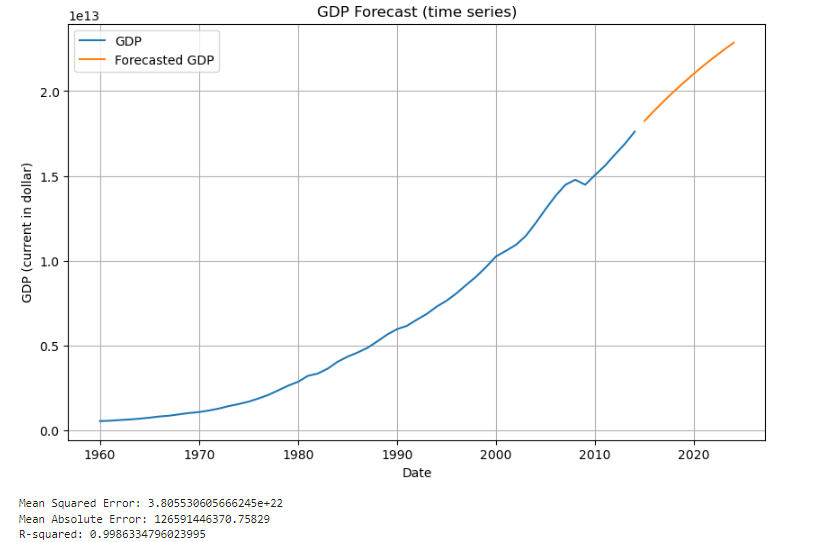
Figure 1: Figure with short caption(data from 1)

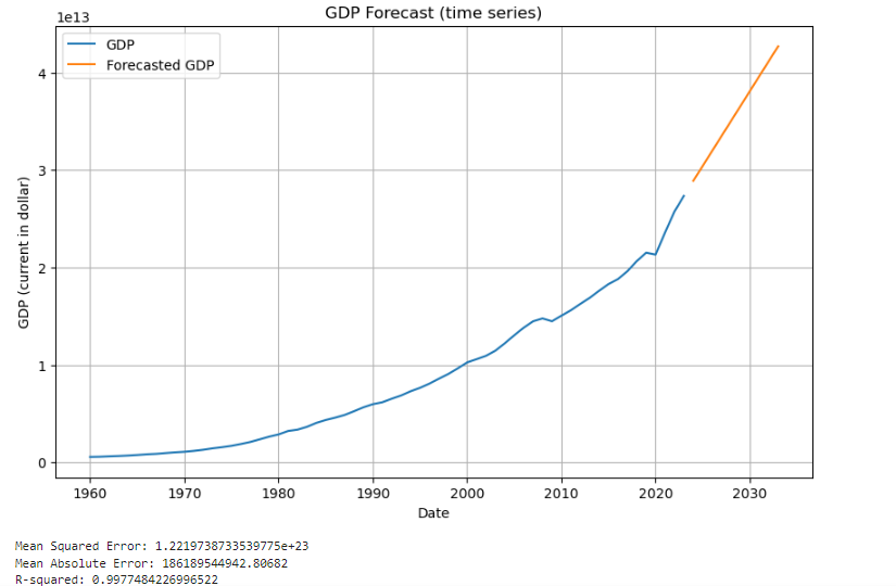
Figure 2: Figure with short caption (data from 1)

The figure shows us the most basic data visualization information, allowing us to clearly see the predicted trends and results. The x-axis represents time, and the y-axis represents GDP in U.S. dollars. There are also three parameters that need to be compared, calculated based on the predicted content. It can be clearly seen that for the time series model, that is, the prediction made by the ARIMA model, its MSE value is approximately within the range.3.8e22 to 1.22e23. MSE measures the average squared difference between actual and predicted values, and in this case its value is low enough, meaning more accurate predictions. Generally speaking, this error is enough to better reflect the prediction made by the model and achieve good results. The next value to consider is MAE, which ranges from 1.26e12 USD to 1.86e12 USD in the ARIMA model. This means that the difference between forecasted GDP and actual GDP is, on average, no more than this range in each condition. This can also illustrate the accuracy of this model. The last one is the R² values. the R² values in the ARIMA model are high. In the first time series forecast shows an R² of 0.9986, which means that nearly 99.86% of the variance in GDP can be explained by the ARIMA model. Next, look at the comparison between the predicted part and the actual part in the figure. It can be clearly seen that within the range of the above three values, the prediction of ARIMA is very consistent with the trend of actual GDP. The accuracy of the predictions made for the next ten years in the second picture cannot be directly visualized, but these three values give a certain reference.

Next is the analysis of the panel data model. The panel data model predicts the GDP of the United States in the next few years, from 2023 to 2030. At the same time, the model also uses the GDP and government expenditure data of three countries, such as the U.S. stock market, Japan, and the United Kingdom, as a reference to make past GDP fittings.

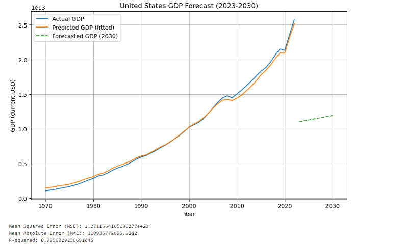
Figure 3: Figure with short caption (data from 1)

According to the calculation results of the model in the figure, we can see that the difference between MSE and time series models is not large, both of them are around 1.3e+23, basically within that interval. But the difference in the subsequent MAE is very large, for the second model, the MAE are almost twice as the time series model. It can clearly see from the figure that although the GDP fitting from 1970 to 2023 is very good, the subsequent predictions have no reference value. This means that its accuracy cannot be used to make any reference. And just because of that, although its R² is within the normal range, R² measures how well the model fits the historical data it was trained on, but it doesn't always reflect future prediction performance. It can be seen from here that the results obtained through panel data model analysis are more inclined to analyze multiple countries and the impact of multiple economic indicators on GDP.

The most critical advantage of time series models is that they are very good at making predictions about a single economic attribute of a single country. Because it can accurately capture historical trends. For example, the prediction of U.S. GDP just shown. The prediction made by this model is very consistent with the trend of historical GDP. It helps “capture the dynamic nature of relationships”.[6] But at the same time, this also gives this model a disadvantage, that is, the model cannot combine various other factors, such as government spending and the GDP of other countries, etc. In other words, it cannot handle more complex calculations. Another limitation of time series models is the reliance on the stationarity of data. “They assume linearity, stationarity, and constant coefficients over time, which may not hold in all cases”. [6] A When data is non-stationary, The accuracy of forecasts may be affected. “Statistical models that are used in forecasting future values of economic time series may not be too useful in predicting a specific event, like a recession”. [7] Panel data models are very helpful for comparing the GDP of multiple countries. When processing different data from multiple countries, such as household expenditures, import and export amounts, and GDP, this model can perform multi-dimensional comparisons of the above data. “Panel data usually give the researcher a large number of data points…hence improving the efficiency of econometric estimates.” [8] However, this model relies heavily on huge data, and at the same time takes into account the mutual influence of each data, and needs to create a good comparison environment. At the same time, the calculation cost and time cost will increase. These factors need to be considered when making predictions in reality.

It is also obvious that this model is not very suitable for predicting the future. In order to make a more accurate prediction rather than fitting it with past data, it may need to add other variables, more data or Simultaneous analysis using time models.

4. Conclusion

Time series models and panel data models are used in comparisons of forecasting future GDP. It is concluded that the ARIMA model is used in economic forecast analysis, such as the future GDP of the United States. Although the forecast numbers are not that precise, they are very consistent with what actually happened in terms of trends. It captures the characteristics and trends of historical data very well and makes a sufficiently accurate analysis. However, it is less capable when dealing with complex multivariate relationships. This model has limitations when dealing with multiple countries or when in needs of joining multiple data for analysis together. Therefore, it is a better choice to use this model when analyzing single data without considering other influencing factors. On the other hand, panel data analysis provides a very good historical data fit by combining the GDP data of multiple countries and various other factors including government expenditures, import and export quotas, etc., which can be used to analyze other economic data and GDP. The relationship is very suitable. However, it demands a larger data set, increased computational resources, and does not provide the same prediction accuracy when applied to future GDP trends. Ultimately, it can be concluded that time series models are better suited for simpler, single-variable predictions, while panel data models are more appropriate when analyzing broader, multi-variable economic scenarios, although with some limitations in forecasting future trends.

References

[1]. World Bank. (2023). GDP (current US$) – US, British, Japan. World Bank Open Data. https://data.worldbank.org/indicator/NY.GDP.MKTP.CD?end=2023&locations=JP&start=1960&view=chart
[2]. ox, G. E. P., Jenkins, G. M., Reinsel, G. C., & Ljung, G. M. (2015). Time Series Analysis: Forecasting and Control. Wiley.
[3]. Baltagi, B. H. (2005). Econometric Analysis of Panel Data (3rd ed.). Wiley.
[4]. Hodson, T. O. (2022). Root-mean-square error (RMSE) or mean absolute error (MAE): When to use them or not. Geoscientific Model Development, 15, 5481-5487. https://doi.org/10.5194/gmd-15-5481-2022
[5]. Greene, W. H. (2012). Econometric Analysis (7th ed.). Pearson. https://www.ctanujit.org/uploads/2/5/3/9/25393293/_econometric_analysis_by_greence.pdf
[6]. Kaur, H., & Jagdev, G. (2023). A comprehensive review on time series forecasting techniques. Journal of Emerging Technologies and Innovative Research (JETIR), 10(5), 297-305. https://www.jetir.org/papers/JETIR2305G16.pdf
[7]. Del Negro, M. (2001). Turn, turn, turn: Predicting turning points in economic activity. Economic Review, Federal Reserve Bank of Atlanta, 86(3), 1-12. https://www.newyorkfed.org/medialibrary/media/research/economists/delnegro/delnegro1.pdf
[8]. Hsiao, C. (2003). Analysis of Panel Data (2nd ed.). Cambridge University Press. https://assets.cambridge.org/052181/8559/sample/0521818559WS.pdf
Cite this article
Chong,K. (2025). Comparative Analysis of Time Series Models and Panel Data Models in Economic Growth Forecasting. Theoretical and Natural Science,83,222-227.
Data availability
The datasets used and/or analyzed during the current study will be available from the authors upon reasonable request.
Disclaimer/Publisher's Note
The statements, opinions and data contained in all publications are solely those of the individual author(s) and contributor(s) and not of EWA Publishing and/or the editor(s). EWA Publishing and/or the editor(s) disclaim responsibility for any injury to people or property resulting from any ideas, methods, instructions or products referred to in the content.
About volume
Volume title: Proceedings of the 4th International Conference on Computing Innovation and Applied Physics
© 2024 by the author(s). Licensee EWA Publishing, Oxford, UK. This article is an open access article distributed under the terms and
conditions of the Creative Commons Attribution (CC BY) license. Authors who
publish this series agree to the following terms:
1. Authors retain copyright and grant the series right of first publication with the work simultaneously licensed under a Creative Commons
Attribution License that allows others to share the work with an acknowledgment of the work's authorship and initial publication in this
series.
2. Authors are able to enter into separate, additional contractual arrangements for the non-exclusive distribution of the series's published
version of the work (e.g., post it to an institutional repository or publish it in a book), with an acknowledgment of its initial
publication in this series.
3. Authors are permitted and encouraged to post their work online (e.g., in institutional repositories or on their website) prior to and
during the submission process, as it can lead to productive exchanges, as well as earlier and greater citation of published work (See
Open access policy for details).