1. Introduction

Differential equations are equations involving unknown functions of one or more independent variables and their derivatives. Solving these equations is an extensive topic in various fields such as fluid mechanics and mathematical finance, with new applications continually emerging. Since most differential equations cannot be solved analytically, the advent of computers in the mid-1900s eventually led to the development of numerical methods for solving complex equations, such as nonlinear ones or those defined over intricate geometries. Despite the popularity and power of traditional numerical methods involving finite differences and finite elements, limitations of these methods still exist, including having difficulty in handling nonlinear problems and obtaining fast solutions that are precise enough for high-dimensional problems.

The recent resurgence in deep neural networks has opened up a brand new track for numerically solving differential equations, especially under circumstances when traditional methods are prone to failure. Specifically, these methods involving neural networks particularly excel in handling nonlinear equations [1] as well as high-dimensional problems [2], and can adapt to complex geometries provided suitable sampling methods are developed [3].

This report will mainly focus on the implementation of solving differential equations with physics-informed neural networks (PINNs). In Section 2, we will introduce some preliminary knowledge relevant to the paper. In Section 3, we will apply the method to solving onevariable ordinary differential equations (ODEs) and discuss the limitations of the approach when solutions with high frequency get involved. The example of a 2D elliptic partial differential equation (PDE) will be displayed in Section 4 together with an extension of the method for solving 3D wave equations. Finally, Section 5 will provide a simple summary of our work with some possible directions for improvements of the method. All codes in this paper are available through the link given in the Appendix.

2. PINNs: Physics-Informed Neural Networks

The Physics-Informed Neural Networks (PINNs) provide a general unsupervised framework for solving differential equations with deep neural networks. Over the recent decades, the method has been widely studied and plays a significant role in solving inverse problems [4] and equation discovery [5]. Given a differential equation with the initial and boundary conditions that the solution satisfies

𝒟[u(x)] = \( f \) (x)forx \( ∈ \) Ω ⊂ \( R \) ^d,(1)

\( {B_{k}} \) [u(x)] = \( {g_{k}} \) (x)forx \( ∈ \) Γ_k ⊂ ∂Ω,(2)

where 𝒟 and \( {B_{k}} \) are differential operators and u(x) is the solution of the equation. PINNs aim to train a neural network, i.e., the output of a multilayer perceptron [6], \( {φ_{θ}} \) (x), to approximate the solution u(x) by minimizing the loss function \( L(θ) \) for a batch of points \( \lbrace {x_{i}}\rbrace _{i=1}^{{N_{p}}} \) ⊂ Ω and \( \lbrace {x_{k,j}}\rbrace _{j=1}^{{N_{b,k}}} \) ⊂ Γ_k ,

\( \underset{θ}{min L}{(θ)}={L_{p}}(θ)+{L_{b}}(θ), \) (3)

\( {L_{p}}(θ)=\frac{1}{{N_{p}}}\sum _{i=1}^{{N_{p}}}{‖ D[{φ_{θ}}({x_{i}})]-f({x_{i}}) ‖^{2}} \) (4)

\( {L_{b}}(θ)=\sum _{k}\frac{{λ_{k}}}{{N_{b,k}}}\sum _{j=1}^{{N_{b,k}}}{‖ B[{φ_{θ}}({x_{k,j}})]-{g_{k}}({x_{k,j}}) ‖^{2}} \) (5)

where λ_k > 0 are pre-specified parameters; \( L \) _p(θ) and \( L \) _b(θ) are referred to as the physics loss and the boundary loss respectively.

To avoid the problem of vanishing gradients, the activation function for each hidden neuron in PINNs should be non-linear and infinitely differentiable. Therefore, the Tanh activation will be chosen for all neurons in hidden layers throughout the experiments in this paper. The derivatives involved in the loss (4) and (5) can be easily obtained using modern learning frameworks such as PyTorch and TensorFlow with automatic differentiation [7, 8].

There are mainly two ways to impose the initial and boundary conditions on the neural network output \( {φ_{θ}} \) . One way is to apply the general formulation (3) and increase the value of λ_k, which leads to PINNs with soft conditions. Another choice is to use the neural network as a part of the solution ansatz so that the network’s output will always satisfy the required boundary (resp., initial) conditions. The latter method eventually results in PINNs with hard conditions.

Once a hard constraint is asserted on the network’s output, the boundary loss \( L \) _b(θ) will no longer be needed as its contribution to the total loss \( L(θ) \) will always be zero. Therefore, the problem will become fully unsupervised and the loss that the network aiming to minimize will be reduced to

\( \underset{θ}{min L}{(θ)}={L_{p}}(θ) \) (6)

if we choose to impose the initial and boundary conditions in a hard manner.

3. Solving Ordinary Differential Equations

3.1. Examples with Dirichlet Boundary Conditions

In this section, we will consider solving the following second-order ODE with Dirichlet boundary conditions (which is also referred to as the type 1 condition throughout this paper for clarity)

\( y \prime \prime (x) = f(x,y,{y^{ \prime }}) \) forx \( ∈ \) \( [a,b] \) ,(7)

\( y(a)={y_{a}} \) and \( y(b)={y_{b}} \) .(8)

PINNs with hard boundary conditions will be applied to obtain the solution of the equation. Let \( {\hat{φ}_{θ}}(x) \) be the original output of the network. The modified output satisfying the Dirichlet boundary conditions is given as

\( {φ_{θ}}(x)={\hat{φ}_{θ}}(x)+\frac{b-x}{b-a}\cdot [ {y_{a}}-{\hat{φ}_{θ}}(a) ]+\frac{x-a}{b-a}\cdot [ {y_{b}}-{\hat{φ}_{θ}}(b) ], \) (9)

with a reduced loss function defined over a series of sampled points \( \lbrace {x_{i}}\rbrace _{i=1}^{{N_{p}}} \) ⊂ \( [a,b] \) given as

\( L(θ)=\frac{1}{{N_{p}}}\sum _{i=1}^{{N_{p}}}{‖φ_{θ}^{ \prime \prime }({x_{i}})-f({x_{i}},{φ_{θ}}({x_{i}}),φ_{θ}^{ \prime }({x_{i}}))‖^{2}}. \) (10)

The test examples we used to illustrate the method in Section 3.4 are listed in Table 1 for a = 0 and b = 1.

Table 1: Known solutions for Dirichlet boundary condition examples.

3.2. Examples with Other Boundary Conditions

The method we used in the previous section for equations with type 1 (Dirichlet) conditions can also be easily generalized to those with other boundary conditions. For example, it can be applied to the same equation with the following type 2 condition

\( y(a)={y_{a}} and y \prime (b)={y_{b}} \) (11)

with ansatz

\( {φ_{θ}}(x)={\hat{φ}_{θ}}(x)+{y_{a}}-{\hat{φ}_{θ}}(a)+(x-a)\cdot [ {y_{b}}-\hat{φ}_{θ}^{ \prime }(b) ], \) (12)

and type 3 condition

y(a) + y^′(a) = \( {y_{a}} and \) y^′(b) = \( {y_{b}} \) ,(13)

with ansatz

\( {φ_{θ}}(x)={\hat{φ}_{θ}}(x)+{y_{a}}-[ {\hat{φ}_{θ}}(a)+\hat{φ}_{θ}^{ \prime }(a) ]+(x-a-1)\cdot [ {y_{b}}-\hat{φ}_{θ}^{ \prime }(b) ]. \) (14)

The loss functions of these formulations remain the same as the one presented in the formula(10). Test examples used for these examples are summarized in Table 2.

Table 2: Known solutions for examples involving conditions of type 2 and 3.

3.3. Example with ODE Systems

Finally, we generalize the method to solve systems of second-order ODEs. Consider the equation (7) and (8) once again with type 1 Dirichlet boundary conditions for some y, f \( ∈ \) \( R \) ^d, d ≥ 2. The solution ansatz and the loss function are the same as the one presented in formulas (9) and (10) in vectorized form. The only change we need to specify is that the output layer of the network now consists of d neurons.

For the numerical experiment, we consider the following system of equations

\( {u^{ \prime \prime }}(x)=x(u-1)-v-{(0.5π)^{2}}sin{(0.5πx)}-2, \) (15)

\( v \prime \prime (x)=v-{x^{2}}(1-x)-6x+2, \) (16)

for x \( ∈ \) [0,1] with y(x) = [u(x),v(x)]^T under the Dirichlet boundary condition. The solution of the system is now given by u(x) = x(1-x) + sin(0.5 \( π \) x) and v(x) = x²(1 − x).

3.4. Numerical Results

Solutions of the sample equations listed in Table 1, Table 2 and equations (15) – (16) are obtained by training a simple 3-layer neural network with only one hidden layer composed of 50 neurons using the Adam optimizer with a batch size of 32 [9]. For each model, only 1000 points (2000 points for solving the ODE system) are sampled from the interval.

For the convenience of comparing the convergence of solving different equations, the L₂ losses L₂(θ) are recorded instead of the physics loss \( L \) _p, defined as

\( {[{L_{2}}(θ)]^{2}}= {∫_{Ω}}{‖{φ_{θ}}(x) - {y_{true}}(x) ‖^{2}} dx \) (17)

The final results are displayed in the above Figure 1. Note that for most of the examples where the true solutions are monotonic functions over the target interval, the method performs a rapid convergence and achieves an accuracy below 10⁻² within only 100 training epochs. However, for a solution with a relatively high latent frequency, for instance, y₄, the method tends to converge in a much slower way.

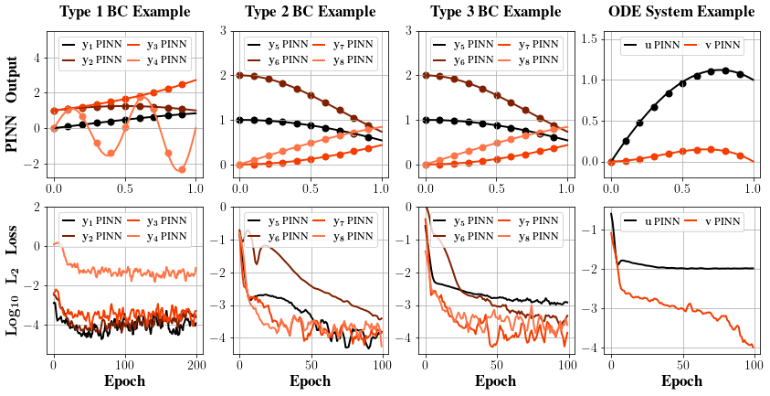
Figure 1: Solutions of Section 3 sample equations generated by PINNs with dots in figures representing the exact value.

3.5. Scaling to Higher Frequencies

In previous examples, we notice that the PINNs tend to converge faster for functions with lower frequencies. Indeed, literature suggests neural networks prioritize learning lower-frequency functions [10]. Furthermore, the capability of these networks to fit high-frequency functions is also bounded by the number of neurons and trainable parameters.

In fact, once the solution involves high-frequency terms, regular PINNs may take a significant amount of time to converge to adequate accuracy even for relatively simple equations. One solution to this challenge of accelerating convergence when scaling PINNs to higher frequencies is introducing Random Fourier Features (RFF) into the training process [11].

The effect of these Fourier features can be viewed as an additional initialization step for the network input. Instead of passing the value of the independent variables x directly into the network \( {φ_{θ}} \) (x), we first convert the input into a series of triangular signals with a pre-specified, fixed random Gaussian matrix G using the map

RFF(x) = [ cos(2πGx), sin(2πGx) ]^T,(18)

where the components of G are drawn independently from a normal distribution N(0,σ²).

We carry out the numerical experiment to study the effect of such an improvement by considering a simple equation y^′′(x) = −(nπ)²y with Dirichlet boundary conditions imposed over the interval [0,1] whose solution is given by y = sin(nπx). The results are summarized in Figure 2.

The experiment mainly reveals several key observations. First, we see the network converges much faster for y with a lower frequency when n = 1. To achieve convergence for such a function, only a regular PINN with a structure of 3 layers and one hidden layer containing 16 neurons is needed, which in all provides (1 + 1) × 16 + (16 + 1) × 1 = 49 trainable parameters.

However, the structure soon becomes inexpressive for n = 5 as the function’s frequency increases. We see the regular network starts to become expressive again when two more hidden layers are added (5 layers in total) to the architecture, and when the number of neurons for each hidden layer is increased to 32. The number of trainable parameters now becomes (1 + 1) × 32 + (32 + 1) × 32 × 2 + (32 + 1) × 1 = 2209.

In comparison, over two thousand new parameters are added to the model to strengthen the expressiveness of the network, while the frequency only increases from 0.5 to 2.5. Luckily, the situation can be alleviated by adding Fourier features to the network structure and evaluating \( {φ_{θ}} \) (RFF(x)) instead. With a Gaussian matrix G sampled from R^8×1, the error of the network’s output quickly converges to a scale of O(10⁻²) for a 3-layer network with a hidden layer of width 16. This time, only (2 × 8 + 1) × 16 + (16 + 1) × 1 − 49 = 240 new trainable parameters are needed to strengthen the network expressiveness.

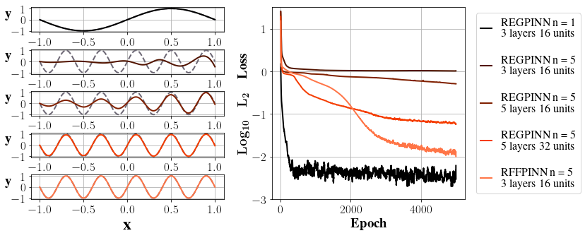
Figure 2: Apply PINNs to high-frequency functions. REGPINN stands for regular PINNs, and RFFPINN represents PINNs with random Fourier features.

4. Solving Partial Differential Equations

4.1. 2D Elliptic Equation

In this section, we apply the PINNs to solving 2D Laplace equations with Dirichlet boundary conditions over rectangular regions Ω = \( [a,b] × [c,d] \) ,

\( {u_{xx}}(x,y)+{u_{yy}}(x,y) = f(x,y) \) for(x,y) \( ∈ \) Ω,(19)

and

\( u(a,y)={u_{a}}(y), u(b,y)={u_{b}}(y), \) (20)

\( u(x,c) ={u_{c}}(x), u(x,d)={u_{d}}(x) \) (21)

To be more specific, we specify the rectangular region to be Ω = [0,1] × [0,1] and set the true solution to be \( {u_{true}} \) ( \( x,y \) ) = sin(2πx)sin(3πy), so that it satisfies the equation for \( f \) ( \( x,y \) ) = −13π² sin(2πx)sin(3πy) and u₀(y) = u₁(y) = u₀(x) = u₁(x) = 0.

The solution ansatz is given in the formula (22) to impose the boundary condition in a hard manner,

\( \begin{matrix} & {φ_{θ}}(x,y) = {\hat{φ}_{θ}}(x,y)+\frac{b-x}{b-a}\cdot [{u_{a}}(y)-{\hat{φ}_{θ}}(a,y)]+\frac{x-a}{b-a}\cdot [{u_{b}}(y)-{\hat{φ}_{θ}}(b,y)] \\ & +\frac{d-y}{d-c}\cdot [{u_{c}}(x)-{\hat{φ}_{θ}}(x,c)]+\frac{y-c}{d-c}\cdot [{u_{d}}(x)-{\hat{φ}_{θ}}(x,d)] \\ & -\frac{(b-x)(d-y)}{(b-a)(d-c)}\cdot [{u_{a}}(c)-{\hat{φ}_{θ}}(a,c)]-\frac{(x-a)(d-y)}{(b-a)(d-c)}\cdot [{u_{b}}(c)-{\hat{φ}_{θ}}(b,c)] \\ & -\frac{(b-x)(y-c)}{(b-a)(d-c)}\cdot [{u_{a}}(d)-{\hat{φ}_{θ}}(a,d)]-\frac{(x-a)(y-c)}{(b-a)(d-c)}\cdot [{u_{b}}(d)-{\hat{φ}_{θ}}(b,d)], \\ \end{matrix} \) (22)

with the loss function

\( L(θ)=\frac{1}{{N_{p}}}\sum _{i=1}^{{N_{p}}}{‖\frac{{∂^{2}}{φ_{θ}}}{∂{x^{2}}}({x_{i}},{y_{i}})+\frac{{∂^{2}}{φ_{θ}}}{∂{y^{2}}}({x_{i}},{y_{i}})-f({x_{i}},{y_{i}})‖^{2}}. \) (23)

We trained a 3-layer network over 2000 sampled points with a batch size of 32 using the Adam optimizer to obtain the solution of the equation (19) – (21); the loss changes are tracked and recorded in the right column of Figure 3 alongside the changes in the L₂ loss.

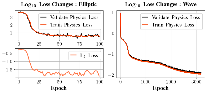
Figure 3: The plots on the left column give the changes in both the physics loss and the L₂ loss while training the PINN to solve the sample elliptic equation (19) – (21); The plots on the right column give the changes in physics losses while training the network to solve the sample wave equation in Section 4.2.

The output of the PINN and its error corresponding to the true solution are shown in Figure 4. For most of the points, the absolute error is controlled within a scale of O(10⁻²), indicating a relatively good approximation.

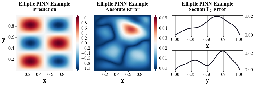
Figure 4: The solution of sample elliptic equation (19) – (21) generated by the PINN (plot 1) with prediction error displayed in plot 2 and 3.

4.2. 3D Wave Equation

The method is also generalized to solve 3D wave equations with 2 spatial dimensions. Consider finding u(x,y,t) over a target region Ω = [0,a] × [0,b] × [0,T] which satisfies the equation,

\( {u_{tt}}={c^{2}}({u_{xx}}+{u_{yy}}) \) \( \) for c > 0,(24)

\( u(0,y,t)=u(a,y,t)=u(x,0,t)=u(x,b,t)=0 \) (25)

\( u(x,y,0)=g(x,y) \) and \( {u_{t}}(x,y,0)=ϕ(x,y) \) .(26)

The analytical solution to this problem can be obtained via Fourier series expansions

\( {u_{true}}(x,y,t)=\sum _{n=1}^{∞}\sum _{m=1}^{∞}sin({μ_{m}}x)sin({ν_{n}}y)[{A_{mn}}cos({λ_{mn}}t)+{B_{mn}}sin({λ_{mn}}t)], \) (27)

where \( {μ_{m}}=\frac{mπ}{a} \) , \( {ν_{n}}=\frac{nπ}{b} \) , \( {λ_{mn}}=c\sqrt[]{μ_{m}^{2}+ν_{n}^{2}} \) , \( {A_{mn}}=\frac{4}{ab}∫_{0}^{a}∫_{0}^{b}g(x,y)sin({μ_{m}}x)sin({ν_{n}}y) dydx \) and \( {B_{mn}}=\frac{4}{ab{λ_{mn}}}∫_{0}^{a}∫_{0}^{b}ϕ(x,y)sin({μ_{m}}x)sin({ν_{n}}y) dydx \) .

This time, the conditions are applied softly to train the network \( {φ_{θ}}(x,y,t) \) , with a loss function

\( \begin{matrix}L(θ)=\frac{{λ_{0}}}{{N_{p}}}\sum _{i=1}^{{N_{p}}}{‖[∂_{tt}^{2}{φ_{θ}}-{c^{2}}(∂_{xx}^{2}{φ_{θ}}+∂_{yy}^{2}{φ_{θ}})]({x_{i}},{y_{i}},{t_{i}})‖^{2}}+\frac{{λ_{1}}}{{N_{b,1}}}\sum _{j=1}^{{N_{b,1}}}{‖{φ_{θ}}(0,{y_{1,j}},{t_{1,j}})‖^{2}} \\ +\frac{{λ_{2}}}{{N_{b,2}}}\sum _{j=1}^{{N_{b,2}}}{‖{φ_{θ}}(a,{y_{2,j}},{t_{2,j}})‖^{2}}+\frac{{λ_{3}}}{{N_{b,3}}}\sum _{j=1}^{{N_{b,3}}}{‖{φ_{θ}}({x_{3,j}},0,{t_{3,j}})‖^{2}}+\frac{{λ_{4}}}{{N_{b,4}}}\sum _{j=1}^{{N_{b,4}}}{‖{φ_{θ}}({x_{4,j}},b,{t_{4,j}})‖^{2}} \\ +\frac{{λ_{5}}}{{N_{b,5}}}\sum _{j=1}^{{N_{b,5}}}{‖{φ_{θ}}({x_{5,j}},{y_{5,j}},0)-g({x_{5,j}},{y_{5,j}})‖^{2}}+\frac{{λ_{6}}}{{N_{b,6}}}\sum _{j=1}^{{N_{b,6}}}{‖{∂_{t}}{φ_{θ}}({x_{6,j}},{y_{6,j}},0)-ϕ({x_{6,j}},{y_{6,j}})‖^{2}}. \\ \end{matrix} \) (28)

Specifically, we solved the equation for a = b = c = T = 1 and trained the network with λ₀ = 5 and λ_k = 20 for k = 1,··· ,6. 2500 points from each of the five boundaries and the interior of the region were sampled to form a training data set of size 15000. The training loss changes were recorded in Figure 3, and the predictions of the PINN are given in Figure 5. Again, the scale of the absolute errors is approximately O(10⁻²).

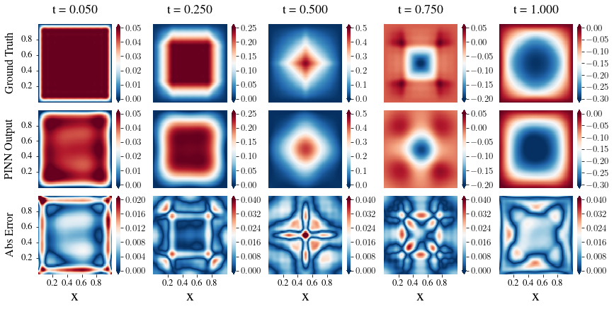
Figure 5: The solution of the sample wave equation generated by the PINN.

5. Conclusion

This paper mainly discusses the application of physics-informed neural networks, i.e., PINNs, to solving differential equations. We first apply the method to ODEs and ODE systems under different types of boundary conditions and find that the solution generated tends to converge slower for high-frequency functions. We then fix the problem and improve the convergence pattern for networks fitting high-frequency solutions by adding random Fourier features to the network structure. Finally, we generalize our work to study the behaviour of PINNs over PDEs with two and three independent variables, where the general absolute errors between the network output and the ground truth are controlled within a scale of O(10⁻²).

However, there are still many aspects that our study fails to cover. For example, most of our example networks are trained under hard conditions. Nevertheless, finding a corresponding solution ansatz can be challenging for complex boundary conditions. Clearly, employing soft conditions is a more versatile approach in the general sense. Also, for more complicated practical problems, PINNs usually suffer from problems of high computational cost and slow convergence.

To increase the flexibility of the method, one possible improvement is to consider conditioned PINNs, where the initial and boundary conditions, as well as other possible features of the equation, are also taken in as part of the network inputs to avoid retraining of similar models [12, 13]. In terms of reducing the computational cost, possible adjustments may be either employing more advanced network architectures [14], or letting networks prioritize learning sample points with higher loss values [15].

References

[1]. M. Raissi, P. Perdikaris, and G.E. Karniadakis. “Physics Informed Deep Learning (Part I): Data-driven Solutions of Nonlinear Partial Differential Equations”. In: ArXiv abs/1711.10561 (2017). url: https: //api.semanticscholar.org/CorpusID:394392 (visited on 05/04/2024).
[2]. W. Ee and B. Yu. “The Deep Ritz Method: A Deep Learning-Based Numerical Algorithm for Solving Variational Problems”. In: Communications in Mathematics and Statistics 6 (2017), pp. 1–12. url: https://api.semanticscholar.org/CorpusID:2988078 (visited on 05/04/2024).
[3]. J. Berg and K. Nystr¨om. “A Unified Deep Artificial Neural Network Approach to Partial Differential Equations in Complex Geometries”. In: ArXiv abs/1711.06464 (2017). url: https://api.semanticscholar. org/CorpusID:38319575 (visited on 05/04/2024).
[4]. J. Adler and O. Oktem. “Solving Ill-posed Inverse Problems Using Iterative Deep Neural Networks”. In:¨ Inverse Problems 33.12 (Nov. 2017), p. 124007. issn: 1361-6420. doi: 10.1088/1361-6420/aa9581. url:http://dx.doi.org/10.1088/1361-6420/aa9581 (visited on 05/04/2024).
[5]. Z. Chen, Y. Liu, and H. Sun. “Physics-informed Learning of Governing Equations from Scarce Data”. In: Nature Communications 12 (2020). url: https://api.semanticscholar.org/CorpusID:239455737 (visited on 05/04/2024).
[6]. F. Rosenblatt. “The Perceptron: A Probabilistic Model for Information Storage and Organization in the Brain.” In: Psychological review 65 6 (1958), pp. 386–408. url: https://api.semanticscholar.org/ CorpusID:12781225 (visited on 05/05/2024).
[7]. A.G. Baydin et al. “Automatic Differentiation in Machine Learning: A Survey”. In: Journal of Machine Learning Research 18 (Apr. 2018), pp. 1–43.
[8]. PyTorch autograd.grad. url: https://pytorch.org/docs/stable/generated/torch.autograd.grad. html (visited on 05/04/2024).
[9]. D.P. Kingma and J. Ba. Adam: A Method for Stochastic Optimization. 2017. arXiv: 1412.6980[cs.LG].
[10]. N. Rahaman et al. “On the Spectral Bias of Neural Networks”. In: International conference on machine learning. PMLR. 2019, pp. 5301–5310.
[11]. M. Tancik et al. “Fourier Features Let Networks Learn High Frequency Functions in Low Dimensional Domains”. In: NIPS ’20., Vancouver, BC, Canada, Curran Associates Inc., 2020. isbn: 9781713829546.
[12]. B. Moseley, A. Markham, and T. Nissen-Meyer. Solving the Wave Equation with Physics-Informed Deep Learning. June 2020. url: https://arxiv.org/abs/2006.11894 (visited on 05/05/2024).
[13]. S. Wang, H. Wang, and P. Perdikaris. “Learning the Solution Operator of Parametric Partial Differential Equations with Physics-Informed Deep Nets”. In: Science Advances 7 (Sept. 2021). doi: 10.1126/sciadv. abi8605.
[14]. Y. Zhu et al. “Physics-Constrained Deep Learning for High-dimensional Surrogate Modeling and Uncertainty Quantification without Labeled Data”. In: Journal of Computational Physics 394 (2019), pp. 56– 81. issn: 0021-9991. doi: https://doi.org/10.1016/j.jcp.2019.05.024. url: https://www. sciencedirect.com/science/article/pii/S0021999119303559 (visited on 05/05/2024).
[15]. C. Wu et al. “A Comprehensive Study of Non-adaptive and Residual-based Adaptive Sampling for PhysicsInformed Neural Networks”. In: Computer Methods in Applied Mechanics and Engineering 403 (Jan. 2023), p. 115671. doi: 10.1016/j.cma.2022.115671.
Cite this article
Dong,C. (2025). Solving Differential Equations with Physics-Informed Neural Networks. Theoretical and Natural Science,87,137-146.
Data availability
The datasets used and/or analyzed during the current study will be available from the authors upon reasonable request.
Disclaimer/Publisher's Note
The statements, opinions and data contained in all publications are solely those of the individual author(s) and contributor(s) and not of EWA Publishing and/or the editor(s). EWA Publishing and/or the editor(s) disclaim responsibility for any injury to people or property resulting from any ideas, methods, instructions or products referred to in the content.
About volume
Volume title: Proceedings of the 4th International Conference on Computing Innovation and Applied Physics
© 2024 by the author(s). Licensee EWA Publishing, Oxford, UK. This article is an open access article distributed under the terms and
conditions of the Creative Commons Attribution (CC BY) license. Authors who
publish this series agree to the following terms:
1. Authors retain copyright and grant the series right of first publication with the work simultaneously licensed under a Creative Commons
Attribution License that allows others to share the work with an acknowledgment of the work's authorship and initial publication in this
series.
2. Authors are able to enter into separate, additional contractual arrangements for the non-exclusive distribution of the series's published
version of the work (e.g., post it to an institutional repository or publish it in a book), with an acknowledgment of its initial
publication in this series.
3. Authors are permitted and encouraged to post their work online (e.g., in institutional repositories or on their website) prior to and
during the submission process, as it can lead to productive exchanges, as well as earlier and greater citation of published work (See
Open access policy for details).