1. Context

1.1. Introduction

Active galactic nucleus (AGN) is a small, compact and bright region in the center of a galaxy that has the highest luminosity. However, with the characteristics shown, the electromagnetic energy emitted was not produced by stars, instead, the radiation is produced by the accretion of matter around a central supermassive blackhole in the galaxy, which devours all matter that gets close to the region. The emitted radiation falls from a wide range of wavelengths, from radio waves to gamma rays, covering across the entire electromagnetic spectrum [1].

The cold matter accrete around the supermassive black hole is based on the conservation of angular momentum and mass. Despite the mass losing angular momentum as it falls into the center of the blackhole, there must be angular momentum transported outward of the black hole through turbulence, hence it redistributes and accretes the cold matter. The turbulence will also heat up the inner region of the disk, which is one of the variables that will be investigated in this paper. The most ubiquitous kind of turbulence that exists in the disk is caused by the Magnetorotational Instability (MRI) [2], which occurs as long as the disk is magnetized and satisfies:

\( \frac{d{Ω^{2}}}{dln{(R)}} \gt 0\ \ \ (1) \)

\( Where {v_{orbital}}=\sqrt[]{\frac{GM}{R}}\ \ \ (2) \)

Here \( Ω \) represents the Keplerian angular velocity of a fluid, and R represents the distance to the rotation centre.

In terms of the mechanism of momentum transport due to magnetic fields, it can be assumed that two arbitrary fluid elements on the inner region of an Keplerian disk can be acted as two mass points connected by a massless spring. The magnetic tension can simply be expressed as the spring tension of the massless spring. From the orbital velocity equation above, the inner fluid element will have a higher orbital velocity than the outer. This makes the ‘massless spring’ to stretch, the closer the region, the faster the orbital speed, the more restoring force there will be for the fluid element to slow down, decreasing the angular momentum. This process will cause the inner fluid element to move to a region with a smaller radius. On the other hand, from the conversation of momentum, the outer fluid element will have a greater angular momentum, and will be pulled outward to an orbit with a greater radius. This model shows that the spring constant in the ‘mass-spring system’ will increase as the two fluid elements move further apart, and gradually cause non-linear growth of perturbation.

In the outer regions of the AGN beyond a critical self-gravitating radius, the disk can also become cold and compact enough to develop gravitational instability or Jeans instability, where the disk tends to collapse vertically from its own self-gravity. The non-linear response from gravitational instability also causes turbulence, to a higher level than MRI such that it can heat the disk towards a marginally gravitationally stable state [3].

However, there is still a limit to the capability of gravito-turbulence in heating the disk against cooling, and beyond a second critical cooling radius, the turbulence/heating level reaches its maximum and runaway cooling is inevitable. In this scenario, the disk will fragment into self-gravitating clumps which leads to intense star formation, and the heat input from these stars may become the dominant heating source instead of turbulence to maintain the disk at a marginally self-gravitating quasi-steady state [4].

Due to different dominating turbulence and heating mechanisms, there are three main regions of the AGN disk, represented by different equations of structure and trends in the turbulent parameter \( α \) .

1.2. The Alpha Disk Model

The alpha disk model was proposed in 1973 by Shakura and Sunyaev [5], with the main property of being thermally and viscously unstable. Physical processes present in the disk leads to turbulence, where the turbulent viscosity of the disk is estimated as equation 3, where \( {c_{s}} \) is the speed of sound, and \( H \) is the scale height, which is represented by equation 4 through vertical hydrostatic equilibrium. Lastly, \( Ω \) is the Keplerian orbital angular velocity, calculated by equation 5, where \( M \) is the central mass of the supermassive black hole (SMBH), and \( R \) is the distance from its center.

\( ν=α{c_{s}}H\ \ \ (3) \)

\( H=\frac{{c_{s}}}{Ω}\ \ \ (4) \)

\( Ω=\frac{{(GM)^{\frac{1}{2}}}}{{R^{\frac{3}{2}}}}\ \ \ (5) \)

There are a few factors to consider in the Alpha Disk Model. Consider an accretion disk that orbits in the \( z=0 \) plane with polar coordinates \( (r, ϕ, z) \) . Assume that the disk is infinitesimally thin, with a negligible mass relative to its SMBH, and is hydrostatic balanced since it accretes slowly. If \( z \lt \lt r \) , the density as a function of z can be written as, \( ρ(z)={ρ_{0}}[-\frac{{z^{2}}}{2{h^{2}}}] \) for a nearly constant sound speed (isothermal limit), which corresponds to the density \( {ρ_{0}} \) at the disk at z = 0, the mid-plane point. From this relationship, the column integrated surface density, \( Σ \) , can be defined by equation 6, and the relation between the surface density and the density at mid-plane in equation 7.

\( Σ=\int _{-∞}^{∞} ρ(z)dz\ \ \ (6) \)

\( {ρ_{0}}=\frac{Σ}{fh}\ \ \ (7) \)

In the isothermal limit the factor \( f = \sqrt[]{2π} \) , but we will generally apply \( f=2 \) , which holds approximately for any self-similar vertical profile. We will also use \( ρ \) to generally refer to the characteristic volume density of the disk.

The presence of viscosity is essential in producing heat when the \( rϕ \) component of the stress tensor, \( {T_{rϕ}} \) , is present between two layers of differentially rotating fluid. This shear due to Keplerian differential rotation contributes to the transport of angular momentum around the SMBH, and can be estimated by equation 8. The product of \( ν \) and \( ρ \) , the density of the fluid, equals to the dynamic viscosity, \( μ \) . \( {T_{rϕ}} \) can therefore be linked with viscosity by equation 8. By introducing an ad hoc assumption from dimensional analysis that the shear stress is proportional to the pressure of the accretion disk, where \( α \) is a turbulent viscosity parameter, shown in equation 9:

\( {T_{rϕ}}=νρr\frac{dΩ}{dr}≈ νρΩ\ \ \ (8) \)

\( {T_{rϕ}}∼αP=αρ{{c_{s}}^{2}}\ \ \ (9) \)

We arrive at the “alpha description” equation 3.

Last but not least, the turbulence strength from a SMBH which is characterized by \( α \) provides a mass flux that accrets towards its center is denoted by \( Ṁ \) , where:

\( Ṁ = 3πα{c_{s}}ΣH\ \ \ (10) \)

This is a constant across distance in a quasi-steady state. The viscous dissipation also provides a heating rate per area, and can be derived by integrating the heating rate per unit volume in an accretion disk by a function of z. The heating rate per unit volume can be expressed by the surface density and the Keplerian shear stress on the \( rϕ \) component:

\( {q_{+}}={T_{rϕ}}r\frac{dΩ}{dr}=μ{(r\frac{dΩ}{dr})^{2}}=\frac{9}{4}μ{Ω^{2}}κ\ \ \ (11) \)

Integrating over \( z \) , the heating rate per unit surface area is:

\( {Q_{+}}=\int _{-∞}^{∞} \frac{9}{4}μ{Ω^{2}}κ dz=\frac{9}{4}νΣ{Ω^{2}}κ\ \ \ (12) \)

In addition, while the disk cools by radiating from two surfaces at the effective temperature, \( {T_{eff}} \) , the temperature will decrease from the midplane due to optical depth \( τ \) in an optically thick environment.

\( {T^{4}}=\frac{3}{8}T_{eff}^{4}τ=\frac{3}{8}T_{eff}^{4}κΣ\ \ \ (13) \)

There is, however, a relation between effective temperature and \( {Q_{+}} \) for optically thick cooling, where \( σ \) is the cross sectional area of interaction:

\( 2σT_{eff}^{4}=\frac{9}{4}νΣ{Ω^{2}}κ\ \ \ (14) \)

2. Mathematical Derivations

2.1. The Master Equation Sets and Three Disk Regions

Before giving a description of the model, there are some constants and variables that need to be defined. There are three equations sets for three main regions of the accretion disk, while some equations apply to more than one region.

• \( \frac{{σ_{SB}}}{c}=a \) , the radiation constant

• \( \frac{{k_{B}}}{{m_{p}}}=\widetilde{R} \) , which is the molar gas constant

• \( {σ_{SB}} \) is the Stefan-Boltzmann constant

• \( κ=\frac{σ}{μ{m_{p}}} \) is the opacity, which we assume to be a constant in a high temperature region = \( 0.4c{m^{2}}/g \) (electron scattering opacity). In the outer regions of the AGN the temperatures will drop below 10^4-10^3 K, and realistically the opacity will undergo a drop before settling down to the grain opacity ~ \( 1 c{m^{2}}/g \) . To first order we neglect this change and apply \( κ = 0.4c{m^{2}}/g \) throughout our calculations.

Three equations can be formed by eliminating expressions for midplane density and scale height. The equations solve for the surface density, temperature and sound speed as functions of \( R \) , the distance from the center of the SMBH, if alpha is a constant. Extra care is needed in writing the equation of state (or pressure equation) since for hot regions of AGN disks, both radiation pressure

\( {p_{rad}}=\frac{a{T^{4}}}{3}\ \ \ (15) \)

and ideal gas pressure

\( {p_{gas}}=\frac{ρ}{μ}\widetilde{R}T\ \ \ (16) \)

needs to be taken into account. Here we take \( μ=0.6 \) for solar composition gas.

2.1.1. The First Disk Region. The first disk region has Q > 1, where Q is the Toomre's stability criterion. This criterion displays the relationship between parameters of a gaseous accretion disc that is differentially rotating to approximate its stability. With the shear force present, it can act as a stabilizing force, and when Q > 1 , it means the system is stable against collapse.

This region is a hot disk that is gravitationally stable and heated by MRI turbulence. It has minimal turbulence, where the viscosity parameter is roughly a constant [5], with \( {α=α_{min}}∼0.02 \) .

The equations below are the continuity, pressure and energy equation for this region:

\( Ṁ =\frac{3παc_{s}^{2}Σ}{Ω}\ \ \ (17) \)

\( \frac{Σ}{\frac{2{c_{s}}}{Ω}}c_{s}^{2}=\frac{1}{3}{aT^{4}}+\frac{Σ}{\frac{2{c_{s}}}{Ω}}\widetilde{R}\frac{T}{μ}\ \ \ (18) \)

\( \frac{16{σ_{SB}}{T^{4}}}{3κΣ}=\frac{9}{4}(\frac{αc_{s}^{2}}{Ω})Σ{Ω^{2}}\ \ \ (19) \)

2.1.2. The Second Disk Region. The second disk region is marginally gravitationally unstable, so Q is maintained to be a constant [3, 4]. The turbulence, \( α \) , adjusts to the cooling rate, so \( α \) is not a constant, and varies between \( {α_{min}} \) and \( {α_{max}} \) . This region has 4 equations that constrain 4 variables:

Q = 1, so \( \frac{{c_{s}}Ω}{πGΣ}=1 \)

\( Ṁ =\frac{3παc_{s}^{2}Σ}{Ω}\ \ \ (20) \)

\( \frac{Σ}{\frac{2{c_{s}}}{Ω}}c_{s}^{2}=\frac{1}{3}{aT^{4}}+\frac{Σ}{\frac{2{c_{s}}}{Ω}}\widetilde{R}\frac{T}{μ}\ \ \ (21) \)

\( \frac{16{σ_{SB}}{T^{4}}}{3κΣ}=\frac{9}{4}(\frac{αc_{s}^{2}}{Ω})Σ{Ω^{2}}\ \ \ (22) \)

2.1.3. The Third Disk Region. This region has a star-forming accretion disk, where its energy balance needs to be maintained by extra heating mechanisms, giving \( α \) takes its largest value. The extra heating needed to balance cooling is given by star formation so beyond the radius where \( α∼{α_{max}} \) , the disk turbulence is decoupled from the energy equation. In this region, 3 equations and 3 variables apply:

Q = 1

\( Ṁ =\frac{3παc_{s}^{2}Σ}{Ω}\ \ \ (23) \)

\( \frac{Σ}{\frac{2{c_{s}}}{Ω}}c_{s}^{2}=\frac{1}{3}{aT^{4}}+\frac{Σ}{\frac{2{c_{s}}}{Ω}}\widetilde{R}\frac{T}{μ}\ \ \ (24) \)

2.2. Limiting Solutions & General Remarks

Before we present the full numerical solutions that bridge all these regions, we would like to make some general remarks.

• \( Σ \) can be expressed by rearranging equation 24: \( Σ=\frac{ṀΩ}{3παc_{s}^{2}} \)

• The generalized equation 25 can be re-written as \( \frac{Σ}{2{c_{s}}/Ω}c_{s}^{2}=\frac{1}{3}a{T^{4}} \) in the radiation dominated region since \( \frac{Σ}{2{c_{s}}/Ω}\widetilde{R}T/μ \) is out of the limit.

• The equation of \( {T^{4}} \) can be expressed after rearranging and by substituting \( Σ \) : \( \frac{Ṁ{Ω^{2}}}{2παc_{s}}={aT^{4}} \)

• The mass flow rate, \( Ṁ \) , is a constant since the density profile remains unchanged.

The radiation dominated regime of the gravitationally stable region is at very close distance to the SMBH, where the following analytical solutions are presented:

Table 1. Solution A, Limited Solutions for the Gravitationally Stable Region.

In this region, there are some properties displayed which can be verified graphically later. Since \( G \) , \( M \) , \( κ \) , \( α \) , \( π \) and \( {σ_{SB}} \) are constants, it can be deduced that \( {c_{s}}∝{R^{-3/2}} \) , \( T∝{R^{-3/8}} \) , \( Σ∝{R^{3/2}} \) , \( ρ∝{R^{3/2}} \) . The scale height is independent from the mass of the black hole and \( R \) , and the temperature is dependent on the mass flow rate.

As the distance from the center of the SMBH increases to the farthest limit, there is a point where we always enter the outermost star forming region, which introduces a new equation 25 for the region, and forms four new equations for \( {c_{s}} \) , \( Σ \) , \( {T^{4}} \) and \( ρ \) , showing different trends.

\( \frac{{c_{s}}Ω}{πGΣ}=1\ \ \ (25) \)

Table 2. Solution B, Limited Solutions for the Star Formation Region.

In this region, the four sets of equations can show an accurate prediction on several properties of different variables in the region. Firstly, the speed of sound in the star formation disk is independent from R, meaning that it remains unchanged throughout the region. It is also unaffected by the mass of the black hole. Meanwhile, \( T \) and \( Σ \) has a steeper gradient in this region than the radiation dominated regime of the gravitationally stable region. Last but not the least, the volume density, \( ρ \) , is independent from both \( α \) and Ṁ, meaning that the mass flow rate and the maximum turbulence does not affect \( ρ \) .

The limiting solutions above also show trends of the variables. For example, \( Σ \) and \( ρ \) will generally increase in the inner region and decrease in the outer region against R. \( T \) will decrease continuously but at two different rates. \( {c_{s}} \) will decrease at the start and then become a constant in the star forming region. Last but not least, the scale height, \( H \) , is a constant in the radiation domination region, and then increases after.

2.2.1. Radiation vs. Gas Pressure Ratio. The radiation/gas pressure ratio is denoted by \( Π=\frac{{p_{rad}}}{{p_{gas}}}=\frac{a{T^{4}}/3}{\frac{ρ}{μ}\widetilde{R}T}∝\frac{{T^{3}}}{ρ} \) :

In the inner solution, since \( T∝{R^{-3/8}} \) and \( ρ \) is independent of \( R \) , as the distance from the center increases in the region, the radiation pressure/gas pressure will decrease. However in the outer solution, \( {T^{3}}∝{R^{-9/4}} \) and \( ρ∝{R^{-3}} \) , which makes \( Π \) to be proportional to \( {R^{3/4}} \) , hence the radiation pressure/gas pressure will increase across the region. This gives a conclusion that there is a transition region which is sandwiched in between the two regions, where radiation pressure vs gas pressure ratio reaches a minimum and the scaling for temperature/density diverges from these limiting solutions. This will be also tested graphically below.

3. Numerical Solutions

3.1. The Fiducial Case

Full numerical solution for the fiducial case, across different disk regions, is shown with black lines in Figure 3. The parameters are defined as shown:

\( Ṁ = \frac{{M_{⊙}}}{yr}\ \ \ (26) \)

\( M \) = \( 1{0^{8}}{M_{⊙}} \)

\( {α_{min}}=0.01 \)

\( {α_{max}}=0.3 \)

The most inner region of the SMBH is gravitationally stable, and it is entirely heated by MRI turbulence, with \( {α_{min}} \) as a constant at approximately 0.02. With low turbulence, there are some properties displayed in this region which conforms with our solution A) in section 2.2. The scale height, \( H \) , remains constant against R, and the volume density and surface density both have a steady increase until it reaches gravitational instability. However, from ¾ the way out from the gravitational stable region, the rate of increase in surface density slows down, which displays another trend when gas pressure begins to take dominance, but before this transition is complete the disk enters the marginally gravitationally unstable region at ~ 0.01pc.

The disks in the gravitational instability region 2 is heated mainly the gravito-turbulence, where the value of \( α \) varies in the range \( {α_{min}} \lt α \lt {a_{max}} \) . It has a value of Q = 1, full equation displayed in equation 25. This shows that the turbulence can change to accommodate the radiative cooling rate in order to maintain the Q value. Figure 1 shows that the \( α \) increases steeply as the distance from the disk to the center of the SMBH increases in this region between ~ 0.01pc and 0.3pc.

In addition, through Figure 3 it shows that as the disk approaches the gravitationally unstable region, there is a continued decline in the ratio of radiation pressure to gas pressure. This indicates that their values are approaching to be equal, and eventually reaches the minimum at the transition to the third region at ~ 0.3 pc. The scalings are slightly nonlinear because gas pressure and radiation pressure are comparable to each other.

Approaching this radius beyond the point where \( α∼{α_{max}} \) , the disk will fragment and form stars. The turbulence will reach its highest level, where the \( α \) value is fixed at \( {α_{max}} \) . Then cooling remains more efficient than the heating sector, mainly due to the turbulence parameter remaining constant. The outer region is where star formation occurs, hence the stars provide heat. There are several properties that conform to the solution B) in section 2.2 in this region, such as the sound speed converges to a constant, since it is independent of \( R \) , and both the surface and volume density decreases linearly as \( R \) increases.

3.2. Dependence on Ṁ & M

We vary the mass flux and mass of the black hole by an order of 10 to observe the changes of disk profile depending on these two parameters. Four cases with \( Ṁ \) = \( [0.1, 10] \frac{{M_{⊙}}}{yr} \) and \( M=[0.1, 10]{ ×1{0^{8}}M_{⊙}} \) are plotted together with the fiducial cases in Figure 2. The labels indicate their “ \( Ṁ \) ” (accretion rate) and “ \( M \) ” (SMBH mass) ratio with the fiducial case, respectively e.g., Md_1_M_10 means the same accretion rate as the fiducial case but a 10 times larger SMBH mass.

First of all, changing the mass of the black hole changes the location of the star formation disk from the center of the SMBH, and Figure 3 shows that the greater the mass of a black hole, the further away the star formation disk is, and vice versa. As the limiting equations from section 2.2 shows that \( {c_{s}} \) is independent from \( R \) in the star formation region, the point on the graph where \( {c_{s}} \) starts to be constant and can determine its location. For instance, after increasing the mass of the black hole by a factor 10, the point where \( {c_{s}} \) becomes constant changes from ~ 0.3 pc to ~ 0.55 pc. In addition, changing the mass and mass flux also impacts the magnitude of the speed of sound, where changing the mass flux makes greater change in \( {c_{s}} \) . From the equation in section 2.2, If \( R \) is constant, then the sound speed is proportional to \( {M^{1/2}} \) and \( Ṁ \) , therefore the equations conform with the graph shown.

The surface density has similar trends with the volume density, where when the mass flux (accretion rate) is lower, there tends to have a slower increase against \( R \) at the gravitational stable disk. The densities all reach their maximum at the point right before entering the star formation disk, and decrease linearly after that, which conforms to the two limiting equations. Figure 3 shows that the surface density changes slightly more when the mass of the black hole is changed than its mass flux, and this matches with the limiting equations, as it shows that \( Σ \) is proportional to \( {M^{-1/2}} \) or \( Ṁ \) assuming if all other variables are constant. However, surface density and volume density both decrease at the same rate in the star forming region, no matter if the black hole has a different mass flux or mass. The mass flux does not have any impact in the volume density of a black hole in the same region as the equation does not have \( Ṁ \) , and this corresponds to the Solution B) in section 2.2.

The scale height is independent from the mass of the black hole in the gravitationally stable disk, and this is shown in Solution A), which matches with the graph in Figure 3. The graph shows that black holes with mass by a scale factor of 0.1 and 10 from the normal one all have the same scale height from the center of the SMBH until they approach the gravitationally unstable region and they start to separate and increase non-linearly. However, the scale height at very large distances increases linearly and at the same rate for all black holes shown on the graph with different mass fluxes or masses, though it is greater for black holes with greater mass flux or smaller mass. This matches with the limiting solutions, as the scale height is proportional to \( {Ṁ^{1/3}} \) and \( {M^{-1/2}} \) .

The temperature profile mildly increases with larger \( Ṁ \) and \( M \) , but the scalings are non-linear in the middle regions. It is close enough to the SMBH where profiles converge to Solution A) in section 2.2, the temperature converges to the profile for different \( Ṁ \) , and only has a mild positive correlation with \( M \) . Last but not the least, Figure 3 shows that the radiation vs. gas pressure ratio decreases at a constant rate at the start, and then at a different gradient in the gravitational unstable disk, then at the point of reaching a minimum, it increases non-linearly since it enters the star formation disk, which is radiation dominated. The trend and graphics correspond with the conclusions stated earlier, which states that the gas pressure and radiation pressure is approximately equal in the transition region between the gravitationally stable and the star formation region.

3.3. Dependence on \( {α_{max}} \)

There are recent radiation hydrodynamic simulations that suggest the maximum level of turbulence supported by gravitational instability in disks with non-negligible radiation pressure (>~10%) is not as large as gas-only simulations previous literature suggests and may be as low as 0.02 [6]. We have tested \( {α_{max}} \) at three different values (0.3, 0.1, 0.02) for \( M=1{0^{8}} \) and \( Ṁ=0.1 \) , and observe how they depend on the maximum turbulence. The default maximum turbulence is \( {α_{max}}∼0.3 \) . There are some remarkable trends which are observed, and noticeable changes occur from the start of the star formation disk. The temperature continuously decreases as we go further away from the center of a SMBH, however, as it reaches the star formation disk, the temperature decreases at a faster rate, and different maximum turbulence changes the initial temperature at the disk. The lower maximum turbulence, the higher temperature at a certain \( R \) , however the turbulence does not affect the rate of the temperature drop as \( R \) increases.

There are also some similar trends which show that the transition from the gravitationally unstable disk to the star-forming disk is closer with a lower maximum turbulence. For example, the sound speed evidently shows that it approaches zero gradient in a lower \( R \) value at \( {α_{max}}=0.02 \) at \( r∼0.01 pc \) while at \( {α_{max}}=0.3 \) , the gradient turns zero at \( r∼0.05 pc \) . This property also matches to the graphs with other parameters, such as the surface density and the scale height as the gradient changes later for higher \( {α_{max}} \) values. The volume density, however, has the same values throughout the SMBH, unaffected by the maximum turbulence, which conforms with the equations in Sec. 2. Last but not least, the radiation vs. gas pressure ratio also conforms with the conclusions from the limited solutions, which shows that there is a minima which is sandwiched between the gravitational unstable region and the star formation region. It also matches the trend where lower turbulence limit corresponds to a smaller transition region, as the graphs also shows that star formation region begins at \( r∼0.01 pc \) when \( {α_{max}}=0.02 \) , and \( r∼0.05 pc \) when \( {α_{max}}=0.3 \) . We do expect there to be no region 2 if \( {α_{max}} \) = \( {α_{min}}. \)

Because the onset of star formation (or the limit on turbulence parameter) reverses the trend of radiation to gas pressure fraction with respect to radius, an early transition to region 3 at larger radiation pressure fraction (for our low \( {α_{max}} \) values) suggests that the disk may simply not be able to reach low enough radiation pressure fraction in order for a gas pressure supported disk to provide larger levels of turbulence, therefore the low \( {α_{max}} \) solutions will be more realistic.

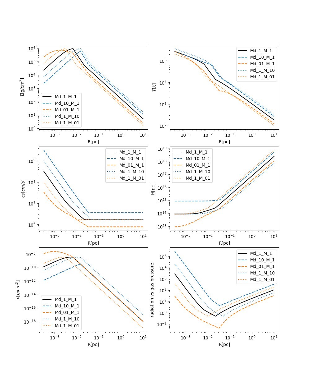
Figure 1. Corresponding Graphs for Different Parameters Against the Distance from the Center of SMBHs with Different Accretion Rates.

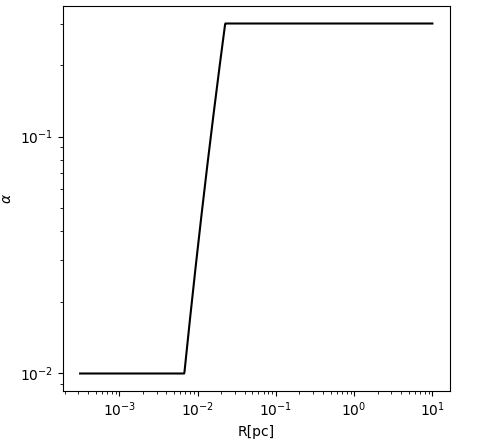
Figure 2. Graph of the Turbulence Constant, \( α \) , against the Distance from the SMBH Center.

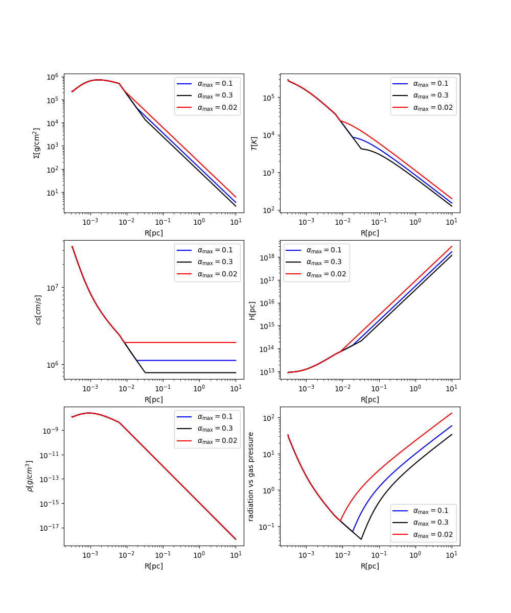
Figure 3. Corresponding Graphs for Different Parameters Against the Distance from the Center of SMBHs with Different Maximum Turbulences.

4. Further Applications

Our disk models can be applied to the modeling of multiple scenarios. First of all, the modeling is directly useful for understanding different temperature profiles of AGN accretion disks probed by reverberation mapping observation [7], and discussing what processes resulted in different dependencies of surface temperature with respect to distance R. Secondly, a disk of stars in the galactic center with a low mutual inclination is suggested to originate from gravitational collapse in an accretion disk while Sgr A* was still in an active phase [8, 9]. In this case, our AGN solutions effectively map out regions of star formation for accretion disk of any \( Ṁ \) and \( M \) , and can be used to study the properties of the fragments or proto-stars as functions of \( R \) in the galactic center as well as in the outskirts of other AGNs.

In addition, another strong evidence for star formation in AGNs lies in the metallicities measured in AGNs. If the metallicities in AGNs are the same as their background environment, it should become more metal poor or “younger” when redshift increases. However, observation of line ratios in AGN spectra show their super-solar abundances do not vary with redshift [10, 11]. This means that stars born in AGNs can pollute their environment through their evolution off the main sequence and their supernovae. Therefore, understanding the disk structure can be useful in calculating the diffusion of elements from embedded stars and how they enhance the metallicity of the whole accretion disk.

Lastly, massive black hole merger components detected in LIGO mergers have been proposed to be of AGN origin [12, 13]. A stellar-mass black hole with approximately 10 solar masses can quickly grow to 30-50 solar mass in an AGN disk either from accreting gas or frequent mergers with their neighbors. This process takes place in the AGN origin, as it is highly dense, lots of stars and black holes can be formed, hence collisions known as galaxy merger occur. In such circumstances, understanding accurate disk structures are crucial in our understanding of the swarm of black holes’ migration and dynamical interaction with the accretion disk, and their thermal feedback onto the disk, in order to predict distinct features of LIGO sources produced from the AGN channel.

5. Conclusions

In this paper, we developed a numerical framework to conveniently generate AGN disk profiles across a wide distance and parameters space, by specifying basic inputs like \( Ṁ \) , \( M \) , \( {α_{max}} \) , \( {α_{min}} \) , and the opacity. Starting from the center of the SMBH, enters the innermost region where the disk will be radiation dominated, and gravitationally stable heated by MRI, to a radiation-dominated, star formation region in the outermost parts. Meanwhile, the middle region displays a minimum of radiation pressure fraction and gravito-turbulence heating which may prevent star formation. We have provided full analytical solutions to the two (closest and furthest) limits of the SMBH, which are verified by numerical solutions of AGN disk that also include the non-linear transition between these two limits. They will be useful in studies of physical processes in AGNs that require modeling of the AGN disk structure.

Acknowledgements

Early this summer, I attended the Astro1107 course in Cornell SCE Pre College Studies; the lectures led by Professor David A. Kornreich have enhanced my background knowledge to complete this research and skills to write a scholarly research paper. I would like to thank my mentor, Mr. Yixian Chen, for encouraging and guiding me in writing this paper and offering me professional advice on using computer programming to display the solutions visually. I also thank his patience and help guiding me through complex Mathematical proofs behind the theories. I would also like to thank my supervisor, Mr. Jeremy Douglas, my Physics teacher at Winchester College, for giving me valuable feedback and continuously challenging my understanding when writing the paper.

References

[1]. Lynden-Bell, D. (1969). Galactic Nuclei as Collapsed Old Quasars. Nature, 223(5207).
[2]. Balbus, S. A. (2003). Enhanced angular momentum transport in accretion disks. Annual Review of Astronomy and Astrophysics, 41(1), 555-597.
[3]. Gammie, C. F. (2001). Nonlinear outcome of gravitational instability in cooling, gaseous disks. The Astrophysical Journal, 553(1), 174.
[4]. Thompson, T. A., Quataert, E., & Murray, N. (2005). Radiation pressure-supported starburst disks and active galactic nucleus fueling. The Astrophysical Journal, 630(1), 167.
[5]. Shakura, N. I., & Sunyaev, R. A. (1973). Black holes in binary systems. Observational appearance. Astronomy and Astrophysics, Vol. 24, p. 337-355, 24, 337-355.
[6]. Chen, Y., Jiang, Y., Goodman, J., & Ostriker, E. (2023). 3D Radiation Hydrodynamic Simulations of Gravitational Instability in AGN Accretion Disks: Effects of Radiation Pressure. The Astrophysical Journal, 948(2), 120
[7]. Cackett, E. M., Bentz, M. C., & Kara, E. (2021). Reverberation mapping of active galactic nuclei: From X-ray corona to dusty torus. Iscience, 24(6).
[8]. Levin, Y., & Beloborodov, A. M. (2003). Stellar disk in the galactic center: a remnant of a dense accretion disk?. The Astrophysical Journal, 590(1), L33.
[9]. Paumard, T., Genzel, R., Martins, F., Nayakshin, S., Beloborodov, A. M., Levin, Y., ... & Sternberg, A. (2006). The two young star disks in the central parsec of the galaxy: properties, dynamics, and formation. The Astrophysical Journal, 643(2), 1011.
[10]. Hamann, F., & Ferland, G. (1999). Elemental abundances in quasistellar objects: star formation and galactic nuclear evolution at high redshifts. Annual Review of Astronomy and Astrophysics, 37(1), 487-531.
[11]. Nagao, T., Marconi, A., & Maiolino, R. (2006). The evolution of the broad-line region among SDSS quasars. Astronomy & Astrophysics, 447(1), 157-172.
[12]. McKernan, B., Ford, K. E. S., Lyra, W., & Perets, H. B. (2012). Intermediate mass black holes in AGN discs–I. Production and growth. Monthly Notices of the Royal Astronomical Society, 425(1), 460-469.
[13]. McKernan, B., Ford, K. E. S., Kocsis, B., Lyra, W., & Winter, L. M. (2014). Intermediate-mass black holes in AGN discs–II. Model predictions and observational constraints. Monthly Notices of the Royal Astronomical Society, 441(1), 900-909.
[14]. Ali-Dib, M., Cumming, A., & Lin, D. N. (2020). The imprint of the protoplanetary disc in the accretion of super-Earth envelopes. Monthly Notices of the Royal Astronomical Society, 494(2), 2440-2448.
Cite this article
Jeff,H.S.C. (2023). Solution of AGN accretion disk structure across a wide range of parameter space. Theoretical and Natural Science,9,187-201.
Data availability
The datasets used and/or analyzed during the current study will be available from the authors upon reasonable request.
Disclaimer/Publisher's Note
The statements, opinions and data contained in all publications are solely those of the individual author(s) and contributor(s) and not of EWA Publishing and/or the editor(s). EWA Publishing and/or the editor(s) disclaim responsibility for any injury to people or property resulting from any ideas, methods, instructions or products referred to in the content.
About volume
Volume title: Proceedings of the 3rd International Conference on Computing Innovation and Applied Physics
© 2024 by the author(s). Licensee EWA Publishing, Oxford, UK. This article is an open access article distributed under the terms and
conditions of the Creative Commons Attribution (CC BY) license. Authors who
publish this series agree to the following terms:
1. Authors retain copyright and grant the series right of first publication with the work simultaneously licensed under a Creative Commons
Attribution License that allows others to share the work with an acknowledgment of the work's authorship and initial publication in this
series.
2. Authors are able to enter into separate, additional contractual arrangements for the non-exclusive distribution of the series's published
version of the work (e.g., post it to an institutional repository or publish it in a book), with an acknowledgment of its initial
publication in this series.
3. Authors are permitted and encouraged to post their work online (e.g., in institutional repositories or on their website) prior to and
during the submission process, as it can lead to productive exchanges, as well as earlier and greater citation of published work (See
Open access policy for details).