1. Introduction

In the medical field, the treatment of a patient often requires the auxiliary cooperation of multiple drugs, and different doses will also affect the final therapeutic effect; In the political field, governance usually requires the introduction of multiple policies, and the intensity of the policies has an important impact on the outcome of governance; In the economic field, multiple complex factors affect stock prices, exchange rates, and so on. In the above areas, different patients, governance regions, and market behaviors will change the results (treatment effect). In these fields, which are awash with large amounts of wealthy observational data, the use of causal inference models to develop the potential of this data is the core purpose of this paper. Although this paper uses the research on precision medicine as an example, it does not deny the scalability of the model in the political and economic fields. In the past, only a single dummy variable was designed to estimate individual treatment effects, and most existing methods predicted counterfactual outcomes based on observed factual data, and few models discussed multi-intervention, continuous numerical dosage for treatment effect estimation. This is the core of this paper.

Estimating the effects of individual treatment effect requires counterfactual results from observational data, which is usually extreme difficult, because unlike experimental data, observational data cannot control variables, that is, there is a causal and correlation relationship between variables [1]. If using traditional machine learning or numerical models to directly predict the target treatment effect, it is likely to introduce heterogeneity bias into the model, resulting in inaccurate estimation of effects. And the traditional individual effect estimation is usually with dummy variable (i.e., with intervention or with no intervention, and only one type of intervention exists), and such simple and direct estimation models cannot be extended to the treatment effect estimation of multiple intervention.

TSGAN (estimating Treatment Spaces using GANs) using GAN estimation to process treatment spaces is a novel GAN network model proposed for this problem. This paper constructs a structure similar to SCIGAN [2]. Inspired by its improvement on counter-factual discriminator, this paper further improve the discriminator, using a series of discriminators in parallel structures to achieve treatment effect space discrimination. Treatment effect space (TES) are a completely new idea proposed in this paper, referring to the individual \( {x_{i}} \) , who owns a space \( {Y_{i}} \) corresponding to different dose levels for each intervention, \( {y_{i}} \) , which will described in detail in following sections. Because of the complexity of treatment effect space, it is not possible to use the ordinary generator of traditional GAN to generate \( TES \) , nor to use its discriminator to distinguish true samples from the generated \( TES \) .

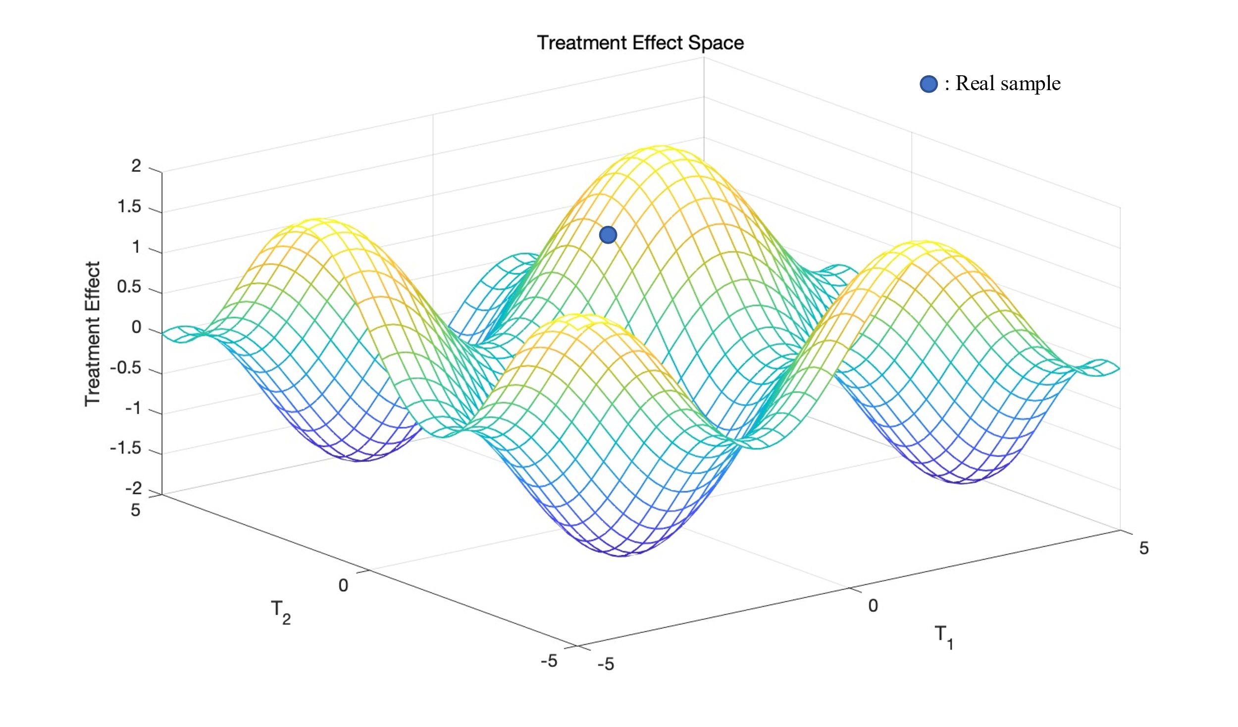
There is only one real sample in the \( TES \) , but there is an entire space of counterfactual. For the generator, if the input has only one random noise \( z \) and some features \( {x_{i}} \) of the individuals, there will be too little information for generator to generate \( TES \) ; For discriminators, there are too many counterfactual samples that need to be discriminated against, and it is difficult to make accurate judgments. In order to solve these two problems, this paper proposes the idea of matching of traditional ITE estimation to solve the problem of generators; Use the method of parallel structural discriminator to solve the problem of discriminators.

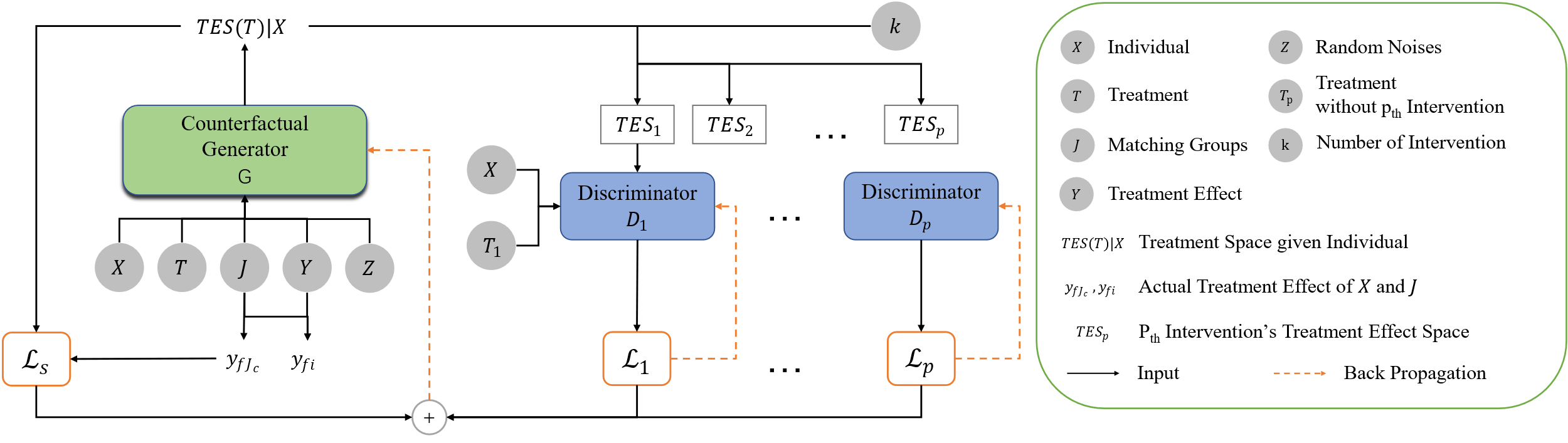
The generator ( \( G \) ) generates \( TES \) corresponding to the input sample and to the nearest neighbor matched group, and each discriminator discriminates the 1-D segmented \( TES \) with individual \( X \) and \( {T_{p}} \) as Input.

In this paper, the construction of the model is described in detail, and the following is expanded in four parts: First, the literature review in individual effect estimation is reviewed and various models are described. Second, the problems that need to be solved in this paper are defined in detail, and the corresponding hypotheses are proposed. Third, the model is constructed part by part, with the generative results and loss functions of each part explained in detail. Forth, Using the TCGA dataset, the data required for model validation in this paper is semi-simulated, and the performance metrics and advantages of the model are compared and explained [2].

2. Literature Review

The study of the treatment effect began as early as the 1980s, and the idea has evolved from the early propensity score matching, which avoids the problem of heterogeneity bias and thus estimates the complier average treatment effect, to the use of machine learning methods such as representation learning and double robust regression [1,3,4].

The core idea of estimating the individual effect is that the treatment effect obtained by different individuals after receiving treatment will vary from person to person, that is, the individual \( x \) has a treatment result \( {y_{f}} \) after receiving treatment \( {t_{f}} \) . How to estimate the treatment effect of \( {y_{cf}} \) , if the individual were to receive treatment \( {t_{cf}} \) . And how to build a model according to \( x, t, {y_{f}}, {y_{cf}} \) to choose the optimal treatment plan for each patient who has not yet received treatment.

At the earliest, research in this area began with numerical imputation based methods, the most common method is called interpolation, including covariate adjustment, backdoor relationship correction, reaction curve estimation and so on [3-6].

After this, a statistical matching method, also known as "strategic downsampling", is often used to balance the inter-group bias between treatment and control groups [7]. Other methods for similar purposes include adjusting backdoor variables, adding instrumental variables, etc. The most notable feature of this type of matching method is that it requires two "regressions" (matches) to estimate the treatment effect.

Today's popular method is causal machine learning, the most commonly used of which is the method of representational learning. The purpose of representation learning is to adjust the covariates through the neural network to balance the distribution of the treatment group and the control group, which are represented by: BNN, SITE, dragonet, TARNet, etc. [8-11].

Another class of methods that use machine learning is to implement counterfactual using adversarial neural networks, which typically also includes an inferential network to generalize the estimation of treatment effects. Representatives are: GANITE and SCIGAN [1,12].

There is also a method of estimating a two-step neural network using a similar DML (double robust machine learning) [13].

The focus of this paper is to explore the estimation of treatment effects under multi-intervention with continuous dosage, of which GANITE and SCIGAN are the ones that realize multiple dose estimation, where this paper is largely inspired by it, and the continuous dosage treatment effect estimation is achieved by DRNets, SCIGAN, etc., of which SCIGAN realizes the treatment effect estimation of continuous dosage with one intervention [1,14] (i.e., patients may receive multiple different dose levels but receive only one treatment at a time, and there is no combination of multiple treatment options). This paper builds on this idea and aimed for estimating treatment effect under multi-continuous dosage intervention.

3. Problem Restatement

Taking precision therapy as an example, assuming that the observed data include the covariates of the patient, the treatment received, and the actual treatment effect, where the covariate is denoted as \( X=\lbrace {x_{i}}\rbrace _{i=1}^{n} \) , treatment received is denoted as \( T=\lbrace {D_{1i}},{D_{2i}},…{D_{ki}}\rbrace _{i=1}^{n} \) , the actual effect of the treatment is denoted as \( {Y_{f}}=\lbrace {y_{fi}}\rbrace _{i=1}^{n} \) . \( k \) is the type of intervention received, \( D \) is the dose of a certain intervention received, \( Y \) is a function of \( T \) and \( X \) . \( {Y_{f}} \) can also be expressed as \( {Y_{f}}=Y(X,{T_{f}}) \) . The observed data samples are \( ({x_{i}},{t_{i}},{y_{i}}) \) . \( X \) is considered as a eigen vector of \( X \) space, \( T \) is a eigen vector of \( T \) space, \( T=\lbrace ({D_{1}},{D_{2}},…,{D_{k}}):{D_{k}}∈{D_{kw}}\rbrace \) . \( {D_{kw}} \) is the dosage range corresponding to the intervention, that is, if a dose range between 0 and 1, then \( {D_{w}}∈[0,1] \) .

As mentioned by PAUL R, the purpose of ITE is to calculate \( ITE=E[Y(t=1)∣X=x]-E[Y(t=0)∣X=x] \) , i.e., the difference in treatment effect between control group and experimental group under conditions of consistent covariate (localized), but this paper studies the treatment effect under multi-intervention with continuous dosage, that is, the treatment effect cannot be expressed by a value. On this basis, we propose the treatment effect space ( \( TES \) ), and our goal is to achieve an unbiased estimation of the TES for each patient based on the observed data given.

\( TES(t)∣[X=x]=E[Y(t)∣X=x] \) (1)

where \( t∈T,x∈X \) . At the same time, to be able to estimate the treatment effect, the data should meet the following assumptions:

Assumption 1 (Overlap):

For all \( ∀x∈X \) , the probability of receiving a certain treatment plan \( p(t|x) \gt 0 \) , \( t∈T \) .

Assumption 2 (Unconfoundedness):

The treatment plan \( {T_{f}} \) , and the treatment effect resulting from that plan \( {Y_{f}} \) , are conditionally independent under the premise given \( X \) .

\( \lbrace Y(t)∣t∈T\rbrace ⊥{T_{f}}∣X \)

3.1. TSGAN Architecture

To achieve the estimation of \( TES \) , we propose a method of using a group-matched modified GAN generator, for each observed data sample with covariates \( {x_{i}} \) , define:

\( {J_{i}}={j_{1}}\cdot {j_{2}},⋯,{j_{c}} \) (2)

Where:

\( {j_{c}}(i)∈argmin{d({x_{j}},{x_{i}})},j∈(1:n) s.t.{ t_{j}}≠{t_{i}} \) (3)

\( C \) is number of sample within the matched group. Since the estimation of the \( TES \) cannot rely solely on unique samples, estimating TES also need \( C \) samples closest to \( {x_{i}} \) as input. This paper refer to the GAN framework proposed in [1] and improve its generators and discriminators so that they can generate and discriminate against treatment effect space. As shown in Figure 2.

3.2. Counterfactual Generator

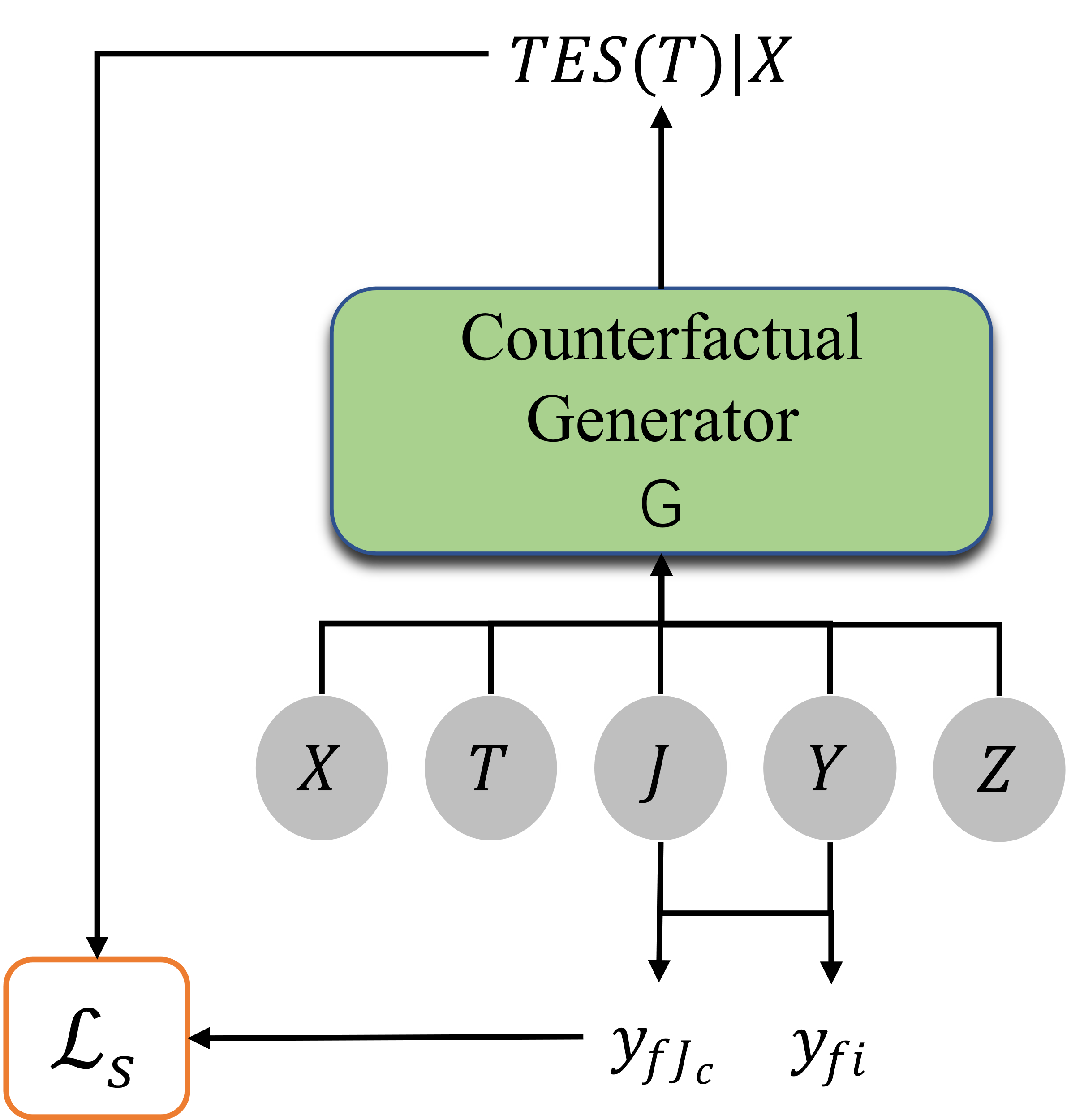
As shown in the Figure 3, counterfactual generator can be represented as: \( X×J×T×Y×Z→{Y^{T}} \) , where the input have covariates \( x∈X \) , the nearest \( C \) sample groups adjacent to x, \( J∈J \) , the treatment effect \( {y_{f}}∈Y \) , the treatment plan \( t∈T \) , and the Gaussian noise \( z∈Z \) . The output \( {Y^{T}} \) is an equation from the treatment space \( T \) to the treatment result \( Y \) , which is the unbiased estimation of \( TES \) :

\( TES(t)=G(x,{t_{f}},{y_{f}},z)(t) \) (4)

Because \( TES \) generated based on the sample’s covariates \( {x_{i}} \) and the \( C \) samples closest to \( x \) , we need to take these elements into account together when considering the generator's loss equation:

\( \begin{array}{c} {L_{s}}(G)=\frac{1}{n}\sum _{i=1}^{n} {|G({x_{i}},{J_{i}},{t_{fi}},{y_{fi}},{z_{i}})({t_{fi}})-{y_{fi}}|^{2}} \\ +\frac{γ}{n\cdot c}\sum _{i=1}^{n} \sum _{c=1}^{C} {|G({x_{i}},{J_{i}},{t_{fi}},{y_{{f_{i}}}},{z_{i}})({t_{f{J_{c}}}})-{y_{f{J_{c}}}}|^{2}} \end{array} \) (5)

3.3. Discriminator

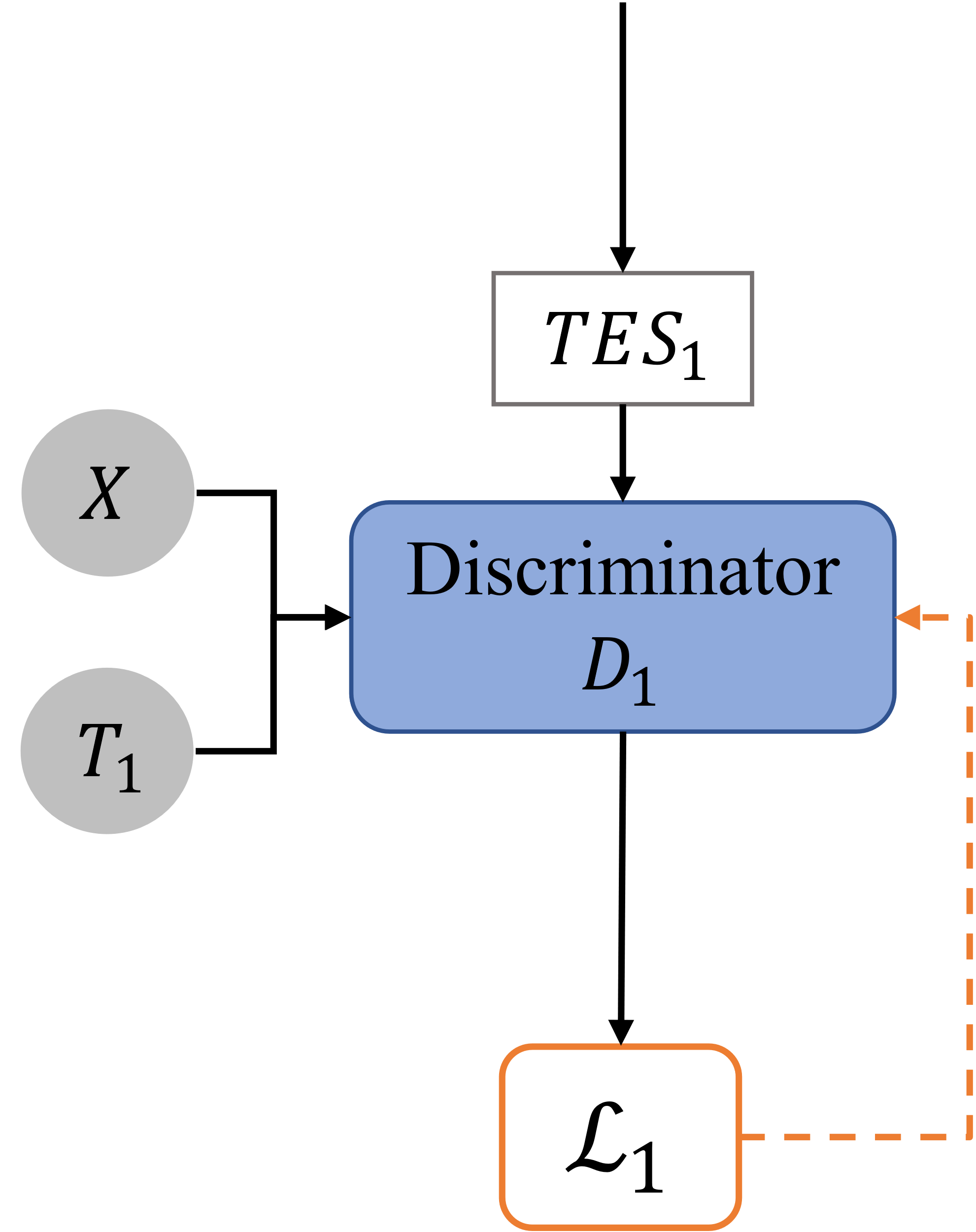
As this paper has always emphasized, traditional GAN discriminators cannot be applied to the TES discriminator. Therefore, this paper tries to reduce the burden on discriminator by dividing the TES by intervention types and apply multiple discriminators. By using paralleled discriminators, each discriminator is responsible for determining 1-D treatment effect space with one intervention.

We discretize the dose of each treatment \( {D_{w}} \) and divide it into \( {n_{w}}∈{Z^{+}} \) dose levels, at this time, \( {D_{kw}}=\lbrace D_{1}^{k},…,D_{{n_{w}}}^{k}\rbrace \) , figuratively speaking, TES is meshed as dosage level is discretized. Our improved discriminator \( {D_{p}} \) takes the covariate \( x \) , partial treatment plan \( {t_{p}} \) , and \( TES \) estimated by the generator as input, where \( {D_{p}} \) is a discriminator specifically for the dose discrimination of the \( {p_{th}} \) intervention, and \( {t_{p}} \) is the treatment plan leave out \( {p_{th}} \) intervention.

\( {t_{p}}=\lbrace ({D_{1}},{D_{2}},…,{D_{p-1}},{D_{p+1}},…,{D_{k}}):{D_{k}}∈ {D_{kw}}\rbrace \) (6)

Define \( {D_{p}}:X×{T_{p}}×TE{S_{p}}→[0,1{]^{{n_{w}}}} \) , where \( TE{S_{p}} \) is the linear space divided from the original \( TES \) when only the dosage in the \( {p_{th}} \) intervention is a variable, and define that the loss function of \( {D_{p}} \) is:

\( {L_{p}}({D_{p}};G)=-\frac{1}{{n_{w}}}\sum _{i=1}^{{n_{w}}} [{I_{({D_{i}}={D_{f}})}}log⁡{D_{p}}(X,{T_{p}},TE{S_{p}})+{I_{({D_{i}}≠{D_{f}})}}log⁡(1-{D_{p}}(X,{T_{p}},TE{S_{p}}))] \) (7)

The output of the discriminator is a probability value between 0 to 1, and for the discriminator given intervention type \( {D_{p}} \) . For each dosage level, the discriminator outputs a probability value, meaning the probability that expected effect given that dosage is trustworthy. So there is a loss function above, where \( {I_{({D_{i}}≠{D_{f}})}}log{{D_{p}}(X,{T_{p}},TE{S_{p}})} \) is the logarithm of the probability at the predicted level as the actual dose level, and the closer the prediction probability is to 1, the smaller the loss; \( {I_{({D_{i}}≠{D_{f}})}}log⁡(1-{D_{p}}(X,{T_{p}},TE{S_{p}})) \) is the logarithm after predicting the wrong dose level, and the closer the prediction is to 0, the smaller the loss.

In summary, the optimization solution of GAN network is as follows:

\( {G^{*}}=arg⁡\underset{G}{min} \sum _{p=1}^{k} L({D_{p}};G)+λ{L_{S}}(G) \) (8)

\( D_{p}^{*}=arg⁡\underset{{D_{p}}}{min} {L_{p}}({D_{p}};{G^{*}}) \) (9)

( \( * \) sign represents the iteration relationship)

3.4. Inference Network

After the generator and discriminator are optimized, we use the generator to generate a corresponding TES for each sample, and then train the inference network using the generated results and the original sample covariate X, so as to predict the TES for new samples.

3.5. Semi-simulated Data Validation

This paper used the Cancer and Tumor Genome Atlas (TCGA) database, with a sample size of over 10,000, covering various omics data such as genome, transcriptome, epigenetics, proteome, etc., providing a comprehensive, multidimensional data. Using the data provided as covariates to construct three treatment plan as shown below:

Table 1. Semi-simulated Data (without interaction terms).

Note: \( v \) is pre-defined simulating terms.

Table 2. Semi-simulated Data (with interaction terms).

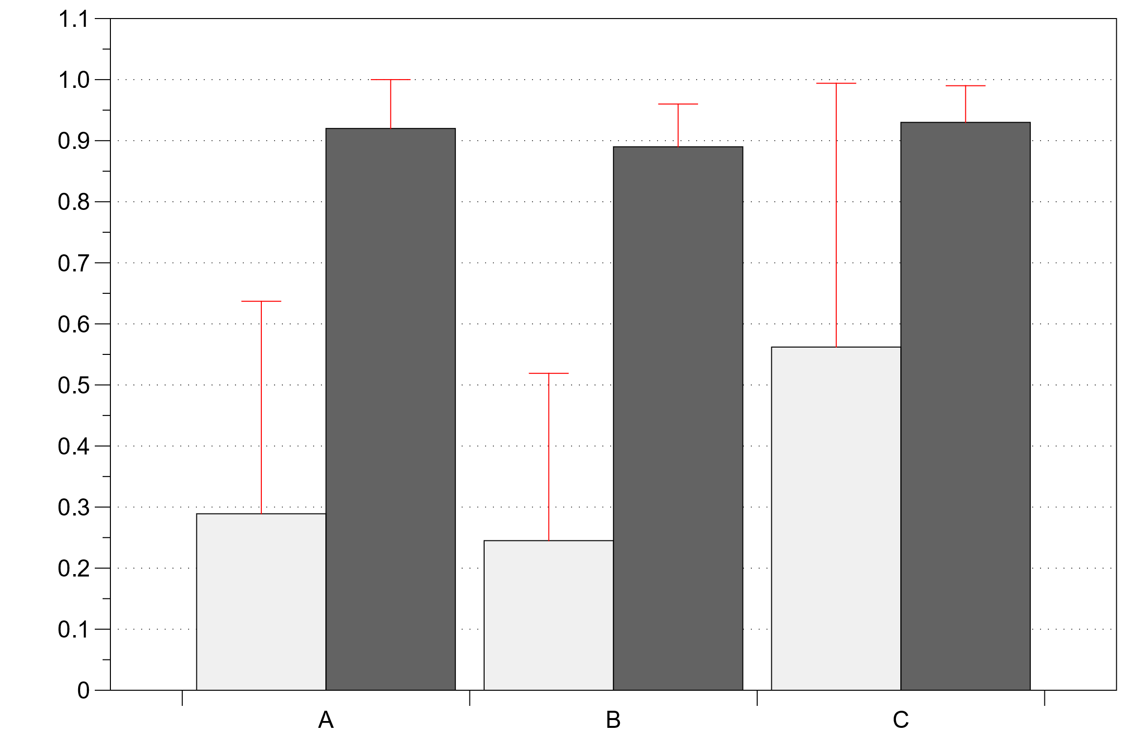
In the validation process, TSGAN performed well without interaction terms, showing more accurate prediction of the optimal dose for treatment plans 1, 2, and 3, and a large nonlinear deviation for 3, but overall more accurate. However, after the addition of interaction terms, the accuracy is greatly reduced, and it is clear that the model needs further improvement to accommodate the interaction effects under multiple treatment regimens.

4. Conclusion

In this paper, the author proposes a method that combines the popular matching idea in traditional ITE estimation with the generative antagonism neural network (GAN) to realize the individual effect estimation under continuous dose intervention and multiple interventions. This work first proposes the idea of processing effect space (TES), and proposes a neural network based on GAN, which uses an improved discriminator. This discriminator uses a different method from the ordinary GAN, and uses multiple discriminators with parallel structure to realize the recognition of real samples in the processing space. In this paper, the discriminator is further improved, and a series of parallel discriminators are used to distinguish the processing effect space. Therapeutic effect space (TES) is a new concept proposed in this paper. Due to the complexity of processing the effect space, it is impossible to use the traditional GAN ordinary generator to generate TES, nor to use its discriminator to distinguish the real samples from the generated TES. In order to solve these two problems, the matching idea of traditional ITE estimation is proposed to solve the generator problem; The parallel structure discriminator is used to solve the discriminator problem. more and better methods and ideas are expected to be found in the future.

References

[1]. PAUL R. ROSENBAUM, DONALD B. RUBIN, The central role of the propensity score in observational studies for causal effects, Biometrika, Volume 70, Issue 1, April 1983, Pages 41–55, https://doi.org/10.1093/biomet/70.1.41
[2]. Bica, Ioana & Jordon, James & Schaar, Mihaela. (2020). Estimating the Effects of Continuous-valued Interventions using Generative Adversarial Networks.
[3]. Austin, Peter C. An introduction to propensity score methods for reducing the effects of confounding in observational studies. Multivariate behavioral research, 46(3):399–424, 2011.
[4]. Funk,MicheleJonsson,Westreich,Daniel,Wiesen,Chris,Sturmer,Til, Brookhart, M Alan, and Davidian, Marie. Dou- ̈ bly robust estimation of causal effects. American journal of epidemiology, 173(7):761–767, 2011.
[5]. Pearl, Judea. Causality. Cambridge university press, 2009.
[6]. Rubin, Donald B. Causal inference using potential outcomes. Journal of the American Statistical Association, 2011.
[7]. Morgan, S. & Winship, C. (2015).Counterfactuals and Causal Inference: Methods and principles for social research. Cambridge: Cambridge University Press. Page 142.
[8]. Fredrik D. Johansson, Uri Shalit, and David Sontag. 2016. Learning representations for counterfactual inference. In Proceedings of the 33rd International Conference on International Conference on Machine Learning - Volume 48 (ICML'16). JMLR.org, 3020–3029.
[9]. Liuyi Yao, Sheng Li, Yaliang Li, Mengdi Huai, Jing Gao, and Aidong Zhang. 2018. Representation learning for treatment effect estimation from observational data. In Proceedings of the 32nd International Conference on Neural Information Processing Systems (NIPS'18). Curran Associates Inc., Red Hook, NY, USA, 2638–2648.
[10]. Shi, Claudia & Blei, David & Veitch, Victor. (2019). Adapting Neural Networks for the Estimation of Treatment Effects.
[11]. Uri Shalit, Fredrik D. Johansson, and David Sontag. 2017. Estimating individual treatment effect: generalization bounds and algorithms. In Proceedings of the 34th International Conference on Machine Learning - Volume 70 (ICML'17). JMLR.org, 3076–3085.
[12]. Yoon, Jinsung et al. “GANITE: Estimation of Individualized Treatment Effects using Generative Adversarial Nets.” ICLR (2018).
[13]. Nair, Naveen & Gurumoorthy, Karthik & Mandalapu, Dinesh. (2022). Individual Treatment Effect Estimation Through Controlled Neural Network Training in Two Stages.
[14]. Patrick Schwab, Lorenz Linhardt, Stefan Bauer, Joachim M Buhmann, and Walter Karlen. Learning counterfactual representations for estimating individual dose-response curves. arXiv, preprint arXiv:1902.00981, 2019.
Cite this article
Lu,H.;Zhang,X.;Bu,E.;Zhu,R.;Jiang,Y.;Tian,P. (2023). TSGAN: Individual treatment effect estimation for multi-intervention with continuous dosage. Theoretical and Natural Science,18,174-181.
Data availability
The datasets used and/or analyzed during the current study will be available from the authors upon reasonable request.
Disclaimer/Publisher's Note
The statements, opinions and data contained in all publications are solely those of the individual author(s) and contributor(s) and not of EWA Publishing and/or the editor(s). EWA Publishing and/or the editor(s) disclaim responsibility for any injury to people or property resulting from any ideas, methods, instructions or products referred to in the content.
About volume
Volume title: Proceedings of the 2nd International Conference on Computing Innovation and Applied Physics
© 2024 by the author(s). Licensee EWA Publishing, Oxford, UK. This article is an open access article distributed under the terms and
conditions of the Creative Commons Attribution (CC BY) license. Authors who
publish this series agree to the following terms:
1. Authors retain copyright and grant the series right of first publication with the work simultaneously licensed under a Creative Commons
Attribution License that allows others to share the work with an acknowledgment of the work's authorship and initial publication in this
series.
2. Authors are able to enter into separate, additional contractual arrangements for the non-exclusive distribution of the series's published
version of the work (e.g., post it to an institutional repository or publish it in a book), with an acknowledgment of its initial
publication in this series.
3. Authors are permitted and encouraged to post their work online (e.g., in institutional repositories or on their website) prior to and
during the submission process, as it can lead to productive exchanges, as well as earlier and greater citation of published work (See
Open access policy for details).