1. Introduction

With the advent of high-performance computers, many numerical methods have been applied to the aerodynamic analysis of airfoils in ideal fluids, and the most widely used method is the panel method. The panel method has been widely used in other fields since it came out, showing strong vitality. Compared with the finite element method and the finite difference method, the advantage of the panel method is that the unknowns are limited to the boundary surface of the solution domain, which greatly reduces the calculation scale. For the basic principle of the panel method, please refer to Lamb, H [1]. The unsteady panel method is a classical boundary element method, which distributes sources and dipole singularities on the surface of the airfoil and object, and the dipole singularities simulate the wake.

Considering the arbitrary motion of the wing, the trajectory of the wake vortex generated by the wing also changes with time. The calculation problem of the wing at this time is an unsteady motion problem. During the unsteady motion of the airfoil, the airfoil circulation changes with time, which will inevitably lead to the equal and opposite direction changes of the circulation of the vented wake vortex. Each individual wake vortex element has an effect on the downwash speed of the wing, but the effect decreases as the wake vortex moves downstream. The lift and drag generated by the wing at a given instant depend on the downwash of the wake vortex system collected by the entire wake. In other words, they are related to the wake vortex system formed by the leakage in the time experience before the instant, the so-called memory effect in a steady motion. The lift and drag of the airfoil are affected by all wake vortices, which is a key characteristic of unstable motion wing issues.

In order to determine the strength of the vortex, the Kutta condition needs to be introduced. Reference [2-4] sets a series of Kutta conditional control points downstream of the airfoil trailing edge, so that the normal velocity on the Kutta conditional control point is 0, and the Kutta conditional control point is taken on the extension surface of the camber of the wing; another method is to equalize the pressure on the pair of control points on the upper and lower surfaces closest to the trailing edge [5,6]. The first method is linear, but the selection of Kutta condition control points is empirical, and the second condition is nonlinear and it needs to be solved iteratively. Robert [7] uses the B-spline method function to represent the source and dipole distribution law of the object surface and the shape of the object surface, and successfully applied it to the solution of the Dirichlet model [8].

Based on the theory of potential flow, this paper summarizes the mathematical models and calculation methods used by different methods to calculate the force of a two-dimensional airfoil under steady motion and unsteady state, including the constant vortex method and the linear vortex method. The influence of different factors on the results is discussed, and the various factors that affect the accuracy of the results are summarized.

2. Calculation of force on airfoil in steady motion

2.1. Problem formulation and basic assumptions

The existing numerical methods for calculating the aerodynamic force of the airfoil can easily meet the accuracy requirements for the calculation of the lift coefficient, but it is not easy to obtain relatively accurate resistance and torque results. There are many factors that affect the numerical results of airfoil aerodynamics. In addition to the factors of the theoretical calculation model, the quality and quantity of meshing and the processing of boundary conditions will affect the accuracy of the calculation results. In order to obtain the best calculation results, various factors that affect the numerical calculation results should be evaluated to find an optimal calculation scheme. In the method presented below, the basic assumption is that the fluid is incompressible and the flow is irrotational.

2.2. Airfoil

Airfoil refers to the cross-sectional shape of an airfoil, sail, propeller, rotor, and turbine. The airfoil can change the direction of the force, for example, it can convert parallel thrust into lift, or horizontal rotational moment into vertical thrust.

The lift of the airfoil mainly comes from the shape of the airfoil and the angle of attack. As shown in Figure 1, the airfoil with a suitable angle of attack will disturb the incoming flow, thereby generating a force in the opposite direction of the disturbance, which is called aerodynamic force. Aerodynamic force can be decomposed into lift and drag. The resultant force perpendicular to the incoming flow direction is called lift force, and the resultant force parallel to the incoming flow direction is called drag force. Most airfoils require a positive angle of attack to generate lift, but cambered airfoils can also generate lift at zero angles of attack. After the incoming flow is disturbed, curved streamlines appear near the surface of the airfoil, so different pressures are generated on the two surfaces of the airfoil. According to Bernoulli's law, the pressure is low where the flow rate is fast, and the pressure is high where the flow rate is slow. Therefore, the lift of the airfoil can be calculated according to the flow rate difference between the upper and lower surfaces. In fact, after introducing the concept of circulation, the lift of the airfoil can be calculated according to the Kutta-Joukowski theorem.

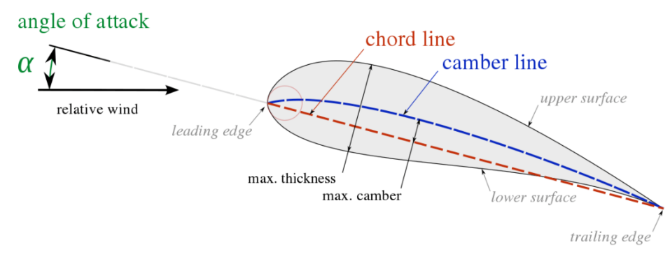
Figure 1. Airfoil nomenclature [9].

2.3. Kinematics definition, governing equations and boundary conditions

Assuming that the perturbation velocity potential generated by the movement of the airfoil is Φ(x,z), the perturbation velocity of the fluid \( V=∇Φ  \) , the velocity potential governing equation is the Laplace equation:

\( {∇^{2}}Φ=0 \) (1)

Boundary conditions include:

(1) The disturbance velocity generated at infinity is zero, that is,

\( ∇Φ=0 \) (2)

(2) The surface of the object is not penetrable, that is,

\( (∇Φ-{V_{A}})∙n=0 \) (3)

Among them, n is the unit normal vector of the object surface, the direction points to the inside of the object, and \( {V_{A}} \) is the incoming flow velocity.

(3) Satisfy the Kutta condition of equal pressure at the trailing edge of the airfoil

\( {P_{m}}={P_{d}}=0 \) (4)

2.4. Numerical method

To solve the problem with the panel method, the first step is to divide the grid. In the calculation mentioned later, the grid is divided into the cosine form. Assuming that the airfoil surface is divided into N units, the number of the unit on the lower surface of the airfoil closest to the tail end is defined as 1, numbered clockwise, and so on. The unit on the airfoil's upper surface closest to the tail end has the number N.

2.4.1. Constant vortex method. The self-induced velocity generated by the constant vortex method at the center of the unit is 0. At the same time, when using the Kutta condition, if using γ₁+γ_N = 0 (γ₁ and γ_N are the distributions of the first and Nth units, respectively vortex strength). At the trailing edge, the lift produced by the higher and lower elements will be cancelled, so if it is N panels, only N-2 equations are available. In order to obtain a definite solution, additional conditions are required, and the boundary conditions need to be modified.

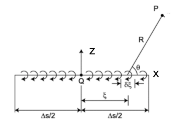
Figure 2. Equal strength vortices distributed along the x-axis [10].

As shown in Figure 2, the induced velocity generated by any panel at a point P in space can be decomposed along the x and z axes of the local coordinate system in the local coordinate system as

\( {u_{p}}=\frac{γ}{2π}[{tan^{-1}}{\frac{z-{z_{2}}}{x-{x_{2}}}}-{tan^{-1}}{\frac{z-{z_{1}}}{x-{x_{1}}}}] \) (5)

\( {w_{p}}=-\frac{γ}{4π}ln{\frac{{(x-{x_{1}})^{2}}+{(z-{z_{1}})^{2}}}{{(x-{x_{2}})^{2}}+{(z-{z_{2}})^{2}}}} \) (6)

\( (\begin{matrix}u \\ w \\ \end{matrix})=(\begin{matrix}cos{α_{i}} & sin{α_{i}} \\ -sin{α_{i}} & cos{α_{i}} \\ \end{matrix})(\begin{matrix}{u_{p}} \\ {w_{p}} \\ \end{matrix}) \) (7)

Convert \( {u_{p}} \) , \( {w_{p}} \) to the velocity in the geodetic coordinate system, there are

\( (u,w)=VOR2DC({γ_{j,}},x,z,{x_{j}},{z_{j}},{x_{j+1}},{z_{j+1}}) \) (8)

To eliminate the element's zero induced velocity to itself, the boundary conditions need to be modified. Inside a closed object

\( ϕ_{i}^{*}=const \) (9)

Since the tangential and normal derivatives of the total velocity potential inside the object are both 0, that is

\( \frac{∂{ϕ^{*}}}{∂n}=\frac{∂{ϕ^{*}}}{∂l}=0 \) (10)

Applying it to each panel, we have

\( {(U+u,W+w)_{i}}∙(cos{α_{i}},-sin{α_{i}})=0 \) (11)

The induced velocity of the J-th panel at the first control point is

\( {(u,w)_{ij}}=VOR2DC({γ_{j}},{x_{1}},{z_{1}},{x_{j}},{z_{j}},{x_{j+1}},{z_{j+1}}) \) (12)

The influence coefficient of unit J of unit strength at the first control point is

\( {a_{ij}}={(u,w)_{ij}}∙(cos{α_{i}},-sin{α_{i}}) \) (13)

α1 is the included angle of the direction of element 1, and the influence coefficient is generally in the form of

\( {a_{ij}}={(u,w)_{ij}}∙(cos{α_{i}},-sin{α_{i}}) \) (14)

Let the incoming flow velocity from a distance be V_A, let

\( RH{S_{i}}=-{(U,W)_{i}}∙(cos{α_{i}},-sin{α_{i}}) \) (15)

A series of equations are obtained through the above process, the unknowns are γ_j ( j=1 to N), and the Kutta condition is γ₁+γ_N = 0. There are N+1 equations and N unknowns, therefore, one equation must be discarded, and the Kutta condition is added to obtain

\( (\begin{matrix}{a_{11}} & ⋯ & ⋯ & ⋯ & {a_{1N}} \\ {a_{21}} & {a_{22}} & ⋯ & ⋯ & {a_{2N}} \\ ⋮ & ⋮ & ⋱ & & ⋮ \\ {a_{N-1,1}} & {a_{N-1,2}} & & ⋱ & {a_{N-1,N}} \\ 1 & 0 & 0 & ⋯ & 1 \\ \end{matrix})(\begin{matrix}{γ_{1}} \\ {γ_{2}} \\ ⋮ \\ ⋮ \\ {γ_{N}} \\ \end{matrix})=(\begin{matrix}{RHS_{1}} \\ {RHS_{2}} \\ ⋮ \\ ⋮ \\ {RHS_{N}} \\ \end{matrix}) \) (16)

To obtain γ_j on each unit, the induced velocity of the airfoil in the flow field can be obtained according to Eqn. (5) and Eqn. (6). Then according to the Bernoulli equation in steady state

\( \frac{p-{p_{∞}}}{p}=-{V_{A}}∙∇ϕ-\frac{1}{2}{(∇ϕ)^{2}} \) (17)

Find the pressure at each control point and integrate it along the airfoil surface

\( F=\oint _{{S_{β}}}pnⅆS \) (18)

The pressure on the airfoil can be obtained.

2.4.2. Linear Vortex Method. Each panel of the airfoil surface is covered in a pattern of linearly shifting vortices. The coordinate system of each element and the induced velocity at a point in space are shown in Figure 3. The vortices at both ends of the first element are set as γ₁ and γ₂, the vortex strengths at both ends of the second unit are γ₂ and γ₃ , and the vortex strength at both ends of the j-th unit are γ_j and γ_j+1 respectively.

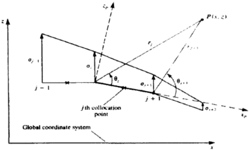
Figure 3. The induced velocity of a linear vortex at any point in space.

The induced velocity generated by a single panel at any point in space can be decomposed along the coordinate axis in the local coordinate system as

\( {u_{p}}=\frac{{γ_{0}}}{2π}[{tan^{-1}}{\frac{z}{x-{x_{2}}}}-{tan^{-1}}{\frac{z}{x-{x_{1}}}}]+\frac{{γ_{1}}}{4π}[zln\frac{{(x-{x_{1}})^{2}}+{z^{2}}}{{(x-{x_{2}})^{2}}+{z^{2}}}+2x({tan^{-1}}{\frac{z}{x-{x_{2}}}}-{tan^{-1}}{\frac{z}{x-{x_{1}}}})] \) (19)

\( {w_{p}}=-\frac{{γ_{0}}}{4π}ln\frac{{(x-{x_{1}})^{2}}+{z^{2}}}{{(x-{x_{2}})^{2}}+{z^{2}}}-\frac{{γ_{1}}}{2π}[\frac{x}{2}ln\frac{{(x-{x_{1}})^{2}}+{z^{2}}}{{(x-{x_{2}})^{2}}+{z^{2}}}+({x_{1}}-{x_{2}})+z({tan^{-1}}{\frac{z}{x-{x_{2}}}}-{tan^{-1}}{\frac{z}{x-{x_{1}}}})] \) (20)

Replace the subscripts 1 and 2 in the equation with j and j+1, and use the vortex strength γ_j and γ_j+1 to represent the trigonometric function, we can get

\( {u_{p}}=\frac{z}{2π}(\frac{{γ_{j+1}}-{γ_{j}}}{{x_{j+1}}-{x_{j}}})ln\frac{{γ_{j+1}}}{{γ_{j}}}+\frac{{γ_{j}}({x_{j+1}}-{x_{j}})+({γ_{j+1}}-{γ_{j}})(x-{x_{j}})}{2π({x_{j+1}}-{x_{j}})}({θ_{j+1}}-{θ_{j}}) \) (21)

\( {w_{p}}=-\frac{{γ_{j}}({x_{j+1}}-{x_{j}})+({γ_{j+1}}-{γ_{j}})(x-{x_{j}})}{2π({x_{j+1}}-{x_{j}})}ln\frac{{γ_{j}}}{{γ_{j+1}}}+\frac{z}{2π}(\frac{{γ_{j+1}}-{γ_{j}}}{{x_{j+1}}-{x_{j}}})[\frac{({x_{j+1}}-{x_{j}})}{z}+({θ_{j+1}}-{θ_{j}})] \) (22)

As can be seen from the above equations, up and wp can be decomposed into the induced velocity γ_j and γ_j+1, respectively. Let

\( u_{p}^{a}=-\frac{z}{2π}(\frac{{γ_{j}}}{{x_{j+1}}-{x_{j}}})ln{\frac{{γ_{j+1}}}{{γ_{j}}}}+\frac{{γ_{j}}({x_{j+1}}-{x_{j}})}{2π({x_{j+1}}-{x_{j}})}({θ_{j+1}}-{θ_{j}}) \) (23)

\( ω_{p}^{a}=-\frac{{γ_{j}}({x_{j+1}}-x)}{2π({x_{j+1}}-{x_{j}})}ln{\frac{{γ_{j}}}{{γ_{j+1}}}}-\frac{z}{2π}(\frac{{γ_{j}}}{{x_{j+1}}-{x_{j}}})[\frac{({x_{j+1}}-{x_{j}})}{z}+({θ_{j+1}}-{θ_{j}})] \) (24)

\( u_{p}^{b}=\frac{z}{2π}(\frac{{γ_{j+1}}}{{x_{j+1}}-{x_{j}}})ln{\frac{{γ_{j+1}}}{{γ_{j}}}}+\frac{{γ_{j+1}}(x-{x_{j}})}{2π({x_{j+1}}-{x_{j}})}({θ_{j+1}}-{θ_{j}}) \) (25)

\( ω_{p}^{b}=-\frac{{γ_{j+1}}(x-{x_{j}})}{2π({x_{j+1}}-{x_{j}})}ln{\frac{{γ_{j}}}{{γ_{j+1}}}} \frac{z}{2π}(\frac{{γ_{j+1}}}{{x_{j+1}}-{x_{j}}})[\frac{({x_{j+1}}-{x_{j}})}{z}+({θ_{j+1}}-{θ_{j}})] \) (26)

we can get

\( {(u,w)_{p}}={({u^{a}},{w^{a}})_{p}}+{({u^{b}},{w^{b}})_{p}} \) (27)

Let

\( (\begin{matrix}u & w \\ {u^{a}} & {w^{a}} \\ {u^{b}} & {w^{b}} \\ \end{matrix})=VOR2DL({γ_{j}},{γ_{j+1}},{x_{j}},{z_{j}},{x_{j+1}},{z_{j+1}}) \) (28)

The induced velocity at the first calculation point can be expressed as

\( {(u,w)_{1}}={({u^{a}},{w^{a}})_{11}}{γ_{1}}+[{({u^{b}},{w^{b}})_{11}}+{({u^{a}},{w^{a}})_{12}}]{γ_{2}}+[{({u^{b}},{w^{b}})_{12}}+{({u^{a}},{w^{a}})_{13}}]{γ_{3}}+…+[{({u^{b}},{w^{b}})_{1N-1}}+{({u^{a}},{w^{a}})_{1N}}]{γ_{N}}+{({u^{b}},{w^{b}})_{1N}}{γ_{N+1}} \) (29)

Let

\( {(u,w)_{11}}={({u^{a}},{w^{a}})_{11}}{γ_{1}} \) (30)

\( {(u,w)_{1,N+1}}={({u^{b}},{w^{b}})_{1N}}{γ_{N+1}} \) (31)

\( {(u,w)_{1,j}}=[{({u^{b}},{w^{b}})_{1, j-1}}+{({u^{a}},{w^{a}})_{1j}}]{γ_{j}} \) (32)

We can get

\( {(u,w)_{1}}={(u,w)_{11}}{γ_{1}}+{(u,w)_{12}}{γ_{2}}+…{(u,w)_{1N+1}}{γ_{N+1}} \) (33)

When γ_j=1, the influence coefficient

\( {a_{ij}}={(u,w)_{i,j}}∙{n_{i}} \) (34)

The free-flow velocity at each vortex element is

\( RH{S_{1}}=-{(U,W)_{i}}∙(cos{α_{i}},sin{α_{i}}) \) (35)

We have N equations, N+1 unknowns, plus the Kutta condition γ_j + γ_j+1 = 1, the linear equation system can be obtained

\( (\begin{matrix}{a_{11}} & {a_{12}} & ⋯ & {a_{1, N+1}} \\ {a_{21}} & {a_{22}} & ⋯ & {a_{2,N+1}} \\ {a_{31}} & {a_{32}} & ⋯ & {a_{3,N+1}} \\ ⋮ & ⋮ & ⋱ & ⋮ \\ {a_{N1}} & {a_{N2}} & ⋯ & {a_{N,N+1}} \\ 1 & 0 & ⋯ & 1 \\ \end{matrix})(\begin{matrix}{γ_{1}} \\ {γ_{2}} \\ {γ_{3}} \\ ⋮ \\ {γ_{N}} \\ {γ_{N+1}} \\ \end{matrix})=(\begin{matrix}{RHS_{1}} \\ {RHS_{2}} \\ {RHS_{3}} \\ ⋮ \\ {RHS_{N}} \\ 0 \\ \end{matrix}) \) (36)

After the vortex strength on each element is solved, the pressure is obtained according to Eqn. (17), and then the total force is calculated according to Eqn. (18).

3. Calculation of force on airfoil in unsteady motion

In many cases, analyzing the aerodynamics of an airfoil requires an unsteady approach, such as:

(1) The motion state of the airfoil changes;

(2) The airfoil moves in an unsteady flow field;

(3) The airfoil moves on the curved surface;

When the two-dimensional airfoil is in an unsteady motion state, the trailing edge of the airfoil will drag out the wake vortex, and the influence of the wake vortex system must be considered when calculating the aerodynamics of the airfoil. In the unsteady state, since the time derivative term of the velocity potential is included in the pressure calculation, the influence of the time derivative of the velocity potential should be considered when introducing the Kutta condition and calculating the pressure distribution. In addition, when considering the influence of complex boundaries, the boundary conditions should also be properly handled.

This chapter discusses the force of the unsteady motion airfoil. First, the mathematical model of the disturbance flow field generated by the two-dimensional unsteady motion airfoil is established, and definite solution conditions are given. Then, equations are discrete, and the singularity elimination equation of the wake vortex-induced velocity is calculated. Finally, the calculation of aerodynamics is discussed, and the factors that affect the accuracy of the results are summarized.

3.1. Basic equations and boundary conditions

Assuming that the perturbation velocity potential generated by the movement of the airfoil is Φ(x,z), the perturbation velocity of the fluid V = ∇Φ, and the velocity potential governing equation is Laplace equation:

\( {∇^{2}}Φ=0 \) (37)

Boundary conditions include:

(1) The disturbance velocity generated at infinity is zero, that is

\( {∇^{Φ}}=0 \) (38)

(2) The surface of the object is not penetrable, that is

\( \frac{∂ϕ}{∂n}|=(U-{V_{A}}+Ω×r)\cdot n \) (39)

Among them, n is the unit normal vector of the object surface, the direction points to the inside of the object, Ω is the rotational angular velocity of the airfoil around the reference point, r is the vector radius of the point on the airfoil surface in the local coordinate system, and V_A is the incoming flow velocity.

(3) Satisfy the Kutta condition of equal pressure at the trailing edge of the airfoil

\( {P_{m}}={P_{d}} \) (40)

where \( {P_{m}} \) and \( {P_{d}} \) represent the pressure at the corresponding points on the upper and lower surfaces of the airfoil trailing edge, respectively.

3.2. Numerical methods

3.2.1. Governing equation. Using the method based on the velocity field, the source and sink are arranged on the airfoil surface \( {S_{B}} \) , and the linear vortex is arranged on the camber line \( {S_{M}} \) ; the wake vortex surface \( {S_{W}} \) is approximated by discrete point vortices. The velocity potential and induced velocity generated by these singularities at any point p in the flow field can be expressed as

\( ϕ(p,t)=\int _{{S_{t}}}σ(q,t)G(p,q)d{s_{q}}+\int _{{S_{M}}+{S_{w}}}Γ(q,t)θ(p,q)d{s_{q}} \) (41)

\( v(p,t)=\int _{{S_{p}}}σ(q,t){∇_{p}}G(p,q)d{s_{q}}+ Γ\int _{{S_{M}}+{S_{w}}}γ(q,t)V(p,q)d{s_{q}} \) (42)

\( σ  \) and Γ are the strength of the distribution vortex on source-sink of the airfoil surface and the strength of the distribution vortex on the wake surface, respectively, where

\( G(p,q)=\frac{1}{2π}ln{r_{p,q}} \) (43)

\( θ(p,q)=\frac{1}{2π}arctan{\frac{{y_{p}}-{y_{q}}}{{x_{p}}-{x_{p}}}} \) (44)

\( V(p,q)=\frac{1}{2π}(\frac{{y_{p}}-{y_{q}}}{r_{pq}^{2}},-\frac{{x_{p}}-{x_{q}}}{r_{pq}^{2}}) \) (45)

\( {r_{p,q}}=\sqrt[]{{({x_{p}}-{x_{q}})^{2}}+{({y_{p}}-{y_{q}})^{2}}} \) (46)

The airfoil surface is divided into N panels, and the camber surface is divided into M panels. When dividing the camber panel, in order to avoid singularity, take the center of the leading circle at the front of the airfoil as the starting point of the panel, and arrange a linear vortex on the camber surface. The strength of the vortex at the starting point is γ₀ = 2γ_f, and the end point is γ(C_f) = 0, so, the strength distribution function of the vortex on the camber surface can be expressed as

\( γ(l)={2_{γ f}}({C_{1}}-1)l{C_{f}} \) (47)

where C_f is the arc length of the camber line, and the total strength of the vortices distributed on the camber line can be expressed as

\( {C_{f}}=\sum _{ j=1}^{ M}\int _{{S_{mj}}}dl  \) (48)

\( {Γ_{f}}=\int _{{S_{mj}}}γ(l)dl={C_{f}}{γ_{f}} \) (49)

The wake surface is approximated by a system of point vortices that are discrete over time steps, with a total strength of Γ_w. Since the unsteady motion is considered, the distribution of source, sink and vortex strength of the above discrete units changes with time, and the time series are expressed as

\( {t_{k}}=kΔt \) (50)

where Δt is the time step. The discrete variable corresponding to the k-th time step is denoted as σ_i^(k), γ_f^(k), Γ_f^(k), Γ_w^(k). In this way, the velocity potential satisfies Eqn. (39) at each control point on the airfoil surface, and the following equations can be obtained:

\( \sum _{j-1 }^{ N}{A_{i,j}}{σ_{j}}+{A_{i,N+1}}∙{γ_{f}}+\sum _{j-1 }^{ k}{C_{i,j}}∙γ_{w}^{(j)}={n_{i}}∙(U-{V_{A}}+Ω∙{r_{i}}) \) (i=1,2,3....N)(51)

where

\( {A_{i,j}}= \int _{{S_{bj}} }\frac{∂}{∂{n_{i}}}G({p_{i}},q)d{s_{q}} \) j=1,2...N(52)

\( {A_{i,N+1}}= {n_{i}}∙\sum _{j=1}^{M}\int _{{S_{bj}} }2({C_{f}}-l)l{C_{f}}∙V({p_{i}},q)d{s_{q}} \) i=1,2....N(53)

\( {C_{i,j}}= {n_{i}}∙V({p_{i}},{q_{w,j}}) \) i=1,2.....N, j=1,2……k(54)

The equation system Eqn. (51) contains N equations and N+3 unknowns, namely the distribution source strength σ_i of the discrete elements on the airfoil surface at the current time step, the distribution vortex strength γ_f on the camber, and the wake vortex strength γ_w^(k) at the current time step. In addition, there is an implicit unknown, which is the position γ_w,k^(k) of the newly generated wake vortex at the current time step. The equation system can be closed by processing the Kutta condition and the wake vortex.

3.2.2. Wake vortices and kutta conditions. The adopted Kutta condition states that identical pressures exist on the top and lower surfaces of the airfoil's trailing edge, which is

\( {P_{u}}-{P_{d}}=0 \) (55)

From Bernoulli’s equation

\( \frac{p-{p_{∞}}}{ρ}=-\frac{∂ϕ}{∂t}+(U-{V_{A}}+Ω×r)∙∇ϕ-\frac{1}{2}{(∇ϕ)^{2}} \) (56)

Plug it into Eqn. (55), we can get

\( \frac{{p_{u}}-{p_{d}}}{ρ}=-\frac{∂{ϕ_{d}}}{∂t}-\frac{∂{ϕ_{u}}}{∂t}+(U-{V_{A}}+Ω×{r_{u}})∙∇{ϕ_{u}}-(U-{V_{A}}+Ω×{r_{d}})∙∇{ϕ_{d}}+\frac{1}{2}[{(∇{ϕ_{d}})^{2}}-{(∇{ϕ_{u}})^{2}}]=0 \) (57)

Among them, the subscript representing the upper surface variable of the airfoil trailing edge is u, the subscript of the lower surface variable of the airfoil trailing edge is d, and r is the vector radius in the local coordinate system. Eqn. (57) contains the square term of the velocity term, so the general iterative solution efficiency is not high, especially when the airfoil motion is complex and the flow field changes drastically, the iterative process is very slow, and even divergence occurs.

The upper and lower surfaces of the trailing edge of the airfoil are very near if the number N of panels on the surface of the airfoil is large enough, then there is

\( {r_{u}}≈{r_{d}}≈\frac{1}{2}({r_{u}}+{r_{d}})={\overline{r}_{e}} \) (58)

where re is the average vector radius at the trailing edge. Plug it into Eqn. (57), then we have

\( \frac{∂({ϕ_{u}}-∂{ϕ_{d}})}{∂t}=\frac{∂{Γ_{f}}}{∂t}≈(U-{V_{A}}+Ω×{\overline{r}_{e}})∙(∇{ϕ_{u}}-∇{ϕ_{d}})+\frac{1}{2}(∇{ϕ_{d}}-∇{ϕ_{u}})(∇{ϕ_{d}}-∇{ϕ_{u}})=(U-{V_{A}}+Ω×{\overline{r}_{e}}-\overline{V})∙(∇{ϕ_{u}}-∇{ϕ_{d}}) \) (59)

Among them, V is the average velocity vector of the upper and lower surfaces of the trailing edge. If the initial value of V is given in the specific solution process, the equation can be linearized and easy to converge.

According to Kelvin's theorem

\( \frac{dΓ}{dt}=\frac{d({Γ_{f}}+{Γ_{w}})}{dt}=0 \) (60)

So at the k-th time step, we have:

\( \frac{d{Γ_{f}}}{dt}=-\frac{d{Γ_{w}}}{dt}≈-\frac{Γ_{w}^{(k)}-Γ_{w}^{(k-1)}}{Δt}=-\frac{γ_{w}^{(k)}}{Δt} \) (61)

From this, it can be obtained

\( Γ_{w}^{(k)}-Γ_{w}^{(k-l)}=γ_{w}^{(k)}=-(Γ_{f}^{(k)}-Γ_{f}^{(k-1)}) \) (62)

Which is

\( Γ_{f}^{(k)}+γ_{w}^{(k)}=Γ_{f}^{(k-1)} \) (63)

From Eqn. (49), we can get

\( {C_{f}}γ_{f}^{(k)}+γ_{w}^{(k)}={C_{f}}γ_{f}^{(k-1)} \) (64)

Eqn. (59) is satisfied at each control point, and the upper and lower surfaces of the trailing edge correspond to the N-th and first panels, respectively, then they can be discretized to obtain:

\( \sum _{j=1 }^{ N}{A_{N+1,j}}{σ_{j}}+{A_{N+1,N+1}}∙{γ_{f}}+\sum _{j-1 }^{ k}{C_{N+1,j}}∙γ_{w}^{(j)}=-\frac{γ_{w}^{(k)}}{Δt} \) (65)

which

\( {A_{N+1,j}}= (U-{V_{A}}+Ω×{\overline{r}_{e}}-\overline{V})∙\int _{{S_{bj}}}[{∇_{p}}G({p_{N}},q)-{∇_{p}}G({p_{1}},q)]d{s_{q}} \) (66)

\( {C_{N+1,j}}= (U-{V_{A}}+Ω×{\overline{r}_{e}}-\overline{V})∙[V({p_{N}},{q_{wj}})-V({p_{1}},{q_{wj}})] \) (67)

\( {\overline{r}_{e}}=\frac{1}{2}({r_{1}}+{r_{N}}) \) (68)

\( \overline{V}=\frac{1}{2}[∇ϕ({p_{t}},t)+∇ϕ({p_{N}},t)] \) (69)

The position of the newly generated wake vortex γ_w,k^(k) can be determined by equation (70).

\( γ_{w,k}^{(k)}={\overline{r}_{e}}-β(U-{V_{A}}+Ω×{\overline{r}_{e}}-\overline{V})Δt \) (70)

Where β is a constant coefficient, and usually, β = 0.4 to 0.6. In this way, the equation system composed of Eqn. (51), Eqn. (64), Eqn. (65) and Eqn. (70) has N+3 equations and N+3 unknowns. The equation system is closed, and it can be iterated. The method is directly solved, that is, given the initial value of V, calculate the coefficients of the equation system, and solve the strength of the source, sink and vortex according to these coefficients (σ₁, σ₂...σ_N), γ_f and γ_w^(k); Calculate the average velocity V of the upper and lower surfaces at the trailing edge using the source-sink and vortex strengths, recalculate the equation coefficients and new source-sink and vortex strengths; repeat this until convergence. The wake vortex needs to be processed before the calculation of the next time step. Without considering the effect of viscosity on the generation and dissipation of vortices, and assuming that the circulation size of the wake vortex remains unchanged and moves at the local speed, the wake vortex at the next moment is described as follows:

\( γ_{w,j}^{(k+1)}=γ_{w,i}^{(k)} \) (71)

\( r_{w,i}^{(k+1)}=r_{w,i}^{(k)}+ΔtV_{w,i}^{(k)} \) (72)

where V_w,i^(k) is the local velocity of the wake vortex numbered i at the current time (time k). Since the calculation of unsteady motion adopts the time stepping method, a large number of new wake vortices are generated at each time step. If there are many time steps or a small time step, so that a large number of wake vortices are generated, the related processing will be taken up a lot of computing time. Due to the limitation of computer memory and computing power, it is necessary to deal with free vortices. There are two commonly used methods. One is to truncate the free vortex system to control the number of free vortex systems; the other is to merge the distant point vortices to reduce the total amount of free vortex systems. The former is that when the number of free vortices exceeds a predetermined value, the initially generated free vortices that are far enough away from the airfoil are discarded, and the latter is to merge the point vortices far away from the airfoil, and combine the distance from the wake vortex system to the airfoil. The free vortices larger than the set value are merged, and then the vortex system is renumbered. The position and intensity of the point vortices after merging are as follows:

\( r_{w,i}^{(new)}=\frac{{γ_{w,i}}}{{γ_{w,i}}+{γ_{w,i+1}}}{r_{w,i}}=\frac{{γ_{w,i+1}}}{{γ_{w,i}}+{γ_{w,i+1}}}{r_{w,i+1}} \) (73)

\( γ_{w,i}^{(new)}={γ_{w,i}}+{γ_{w,i+1}} \) (74)

Eqn. (41) can be used to determine the velocity potential of a location on the airfoil's surface at any time, or it can be obtained by the integral of the speed along the contour of the airfoil, which is

\( ϕ(l)=ϕ({q_{1}})+\int _{{q_{1}}}^{q}v(l)∙dl \) (75)

Among them, Φ(q1) is the velocity potential at point q1 on the lower surface of the airfoil, which has different values at different times, but considering that the constant distribution pressure around the airfoil has no effect on the aerodynamics, the effect of Φ(q1) is ignored in the actual calculation. Then the pressure distribution on the airfoil surface can be obtained according to Bernoulli's equation Eqn. (38). Define the airfoil surface pressure distribution coefficient:

\( {C_{p}}=\frac{p-{p_{∞}}}{0.5ρV_{A}^{2}} \) (76)

The wing force is

\( F=({F_{x,}}{F_{y}})=0.5ρV_{A}^{2}∙\int _{{S_{b}}}{C_{p}}n dS \) (77)

4. Conclusion

This paper first summarizes the force problem of calculating the steady and unsteady motion of two-dimensional airfoils, and the main conclusions are summarized as follows:

First, the numerical method for solving the aerodynamic problem of two-dimensional steady motion airfoil is discussed. For the aerodynamic calculation problem of two-dimensional airfoil, various factors that affect the accuracy of the result in numerical calculation are discussed, that is, the choice of grid division method, the selection of the distribution vortex law of the camber surface, and the selection of the number of meshes; in order to obtain numerical results with higher accuracy, it is best to use an asymmetrically refined mesh division method, and appropriately increase the number of meshes. It is best to use a high-precision vortex distribution law.

Second, the numerical method for solving the aerodynamic problem of two-dimensional unsteady motion airfoil is discussed, and the factors that affect the result, such as the time step, are discussed. For the same airfoil, different time steps have little effect on the results. In the calculation, the time step can be appropriately increased to save the calculation time and improve the calculation efficiency.

References

[1]. Morino, L., Kuo, C.C.: Subsonic potential aerodynamics for complex configurations: a general theory. AIAA Journal 12. (2), 191-197 (1974).
[2]. Labrujere, TH.E., Saaris, CxR.: An calculation subcritical of the pressure distribution on approximate method for wing-body combinations speeds. Agard Conf. Proc. No.71 (1970).
[3]. Kraus, W.: Das MBB-UFE Unterschall Panelverfahren, Report MBB-UFE, 633-70 (1970).
[4]. Robert, P.E., Searis, CxR.: A general method for determining the aerodynamic characteristics of fan-in-wing configurations. Theory and Application, Technical Report, 67-61a (1967).
[5]. Hess, J.L.: The problem of 3-D lifting potential flow and its solution by of surface singularity distributions. Computer Methods in Applied Mechanics and Engineering 4, 283-319 (1974).
[6]. Heckmann, Q., Vitte, W.: Ecoulement & potential tri-dimensional portent. AFITAE Applied Aerodynamics Colloquium (1971).
[7]. Roberts, A., Rundle, K.: Computation of incompressible flow about bodies and thick wings: using the spline mode system. BAC (CAD) Report Aero MA 19, (1972).
[8]. Johnson, F.T., Rubbert, P.E.: Advanced panel-type influence coefficient methods applied to subsonic flows (1975).
[9]. Wikimedia Foundation. (2022, August 17). Airfoil. Wikipedia. Retrieved October 11, 2022, from https://en.wikipedia.org/wiki/Airfoil.
[10]. Bristow, D.R. Recent improvements in surface singularity methods for the flow field analysis about two-dimensional airfoils (1977).
Cite this article
Gao,Y. (2023). Aerodynamic analysis of airfoil in steady and unsteady motion. Theoretical and Natural Science,18,192-203.
Data availability
The datasets used and/or analyzed during the current study will be available from the authors upon reasonable request.
Disclaimer/Publisher's Note
The statements, opinions and data contained in all publications are solely those of the individual author(s) and contributor(s) and not of EWA Publishing and/or the editor(s). EWA Publishing and/or the editor(s) disclaim responsibility for any injury to people or property resulting from any ideas, methods, instructions or products referred to in the content.
About volume
Volume title: Proceedings of the 2nd International Conference on Computing Innovation and Applied Physics
© 2024 by the author(s). Licensee EWA Publishing, Oxford, UK. This article is an open access article distributed under the terms and
conditions of the Creative Commons Attribution (CC BY) license. Authors who
publish this series agree to the following terms:
1. Authors retain copyright and grant the series right of first publication with the work simultaneously licensed under a Creative Commons
Attribution License that allows others to share the work with an acknowledgment of the work's authorship and initial publication in this
series.
2. Authors are able to enter into separate, additional contractual arrangements for the non-exclusive distribution of the series's published
version of the work (e.g., post it to an institutional repository or publish it in a book), with an acknowledgment of its initial
publication in this series.
3. Authors are permitted and encouraged to post their work online (e.g., in institutional repositories or on their website) prior to and
during the submission process, as it can lead to productive exchanges, as well as earlier and greater citation of published work (See
Open access policy for details).